Thermal Analysis of a Disc Brake
| Introduction | Model extensions |
| Axisymmetric Heat Transfer equation | Nomenclature |
| 2D axisymmetric heat transfer model | References |
Introduction
A braking system is generally composed of a brake disc and two brake pads. When braking, the brake pads exerts pressure on the disc to decelerate it. In this process there is a transformation of mechanical energy to thermal energy due to the friction between the pads and the disk. This energy is then dissipated in the material of the disk causing a change in the temperature distribution ![]() in
in ![]() . This notebook demonstrated a transient thermal analysis to calculate the temperature distribution caused by braking. The geometry of the disk and brake pads are mostly rotationally symmetric and an axisymmetric heat transfer analysis will be shown. The model shown is a simplified disc brake that has brake pads all around and that is based on [Adamowicz,2015]. The rotationally symmetric assumption is warranted by the fact that the disk rotates quickly compared to the size of the pads.
. This notebook demonstrated a transient thermal analysis to calculate the temperature distribution caused by braking. The geometry of the disk and brake pads are mostly rotationally symmetric and an axisymmetric heat transfer analysis will be shown. The model shown is a simplified disc brake that has brake pads all around and that is based on [Adamowicz,2015]. The rotationally symmetric assumption is warranted by the fact that the disk rotates quickly compared to the size of the pads.
The phenomenon of heat transfer is described by the heat equation, but in this example can be described by a special case of the heat equation: the axisymmetric form. This can be done because the domain and the boundary conditions are rotationally symmetric about the ![]() -axis. Using an axisymmetric model has the advantage that the computational cost in both time and memory is much less than in the case of solving a 3D heat transfer problem.
-axis. Using an axisymmetric model has the advantage that the computational cost in both time and memory is much less than in the case of solving a 3D heat transfer problem.
Axisymmetric Heat Transfer equation
The axisymmetric heat transfer equation is given as:
where ![]() is the mass density in
is the mass density in ![]() ,
, ![]() is the specific heat capacity in
is the specific heat capacity in ![]() and
and ![]() is the thermal conductivity in
is the thermal conductivity in ![]() .
.
The axisymmetric heat equation uses a truncated cylindrical coordinate system in 2D with independent variables ![]() instead of the cylindrical coordinates
instead of the cylindrical coordinates ![]() . The cylindrical coordinate variable
. The cylindrical coordinate variable ![]() disappears because the system is rotationally symmetric about the
disappears because the system is rotationally symmetric about the ![]() -axis.
-axis.
More information on the axisymmetric heat equation is given in the section Special Cases of the Heat Equation in the heat transfer overview monograph.
Domain
The domain of analysis in this case is an axially symmetric geometry, also known as body of revolution. The sketch below shows the simulation domain which is a rectangular region (disk) and one of the two brake pads.

Revolving the black rectangular region which is the cross section through the brake disk around the ![]() -axis, the axis of revolution, we get the 3D model geometry as seen in the figure below.
-axis, the axis of revolution, we get the 3D model geometry as seen in the figure below.

In the following all length scales are given in meters ![]() . The simulation set up consists of a disk and a pad and there are various symmetries that are exploited. For one we have the rotational symmetry around the
. The simulation set up consists of a disk and a pad and there are various symmetries that are exploited. For one we have the rotational symmetry around the ![]() -axis which allows us to reduce the simulation domain only to a rectangular region corresponding to the axisymmetric section of the annular disc. A second symmetry is indicated by the cut line though the disk. Normally a brake system has a disk and two brake pads acting on the disk from both sides. Due to the second symmetry it is possible to half the disk thickness and only model one pad. The equation is then solved in the reduced disk and the pad is modeled as a boundary condition.
-axis which allows us to reduce the simulation domain only to a rectangular region corresponding to the axisymmetric section of the annular disc. A second symmetry is indicated by the cut line though the disk. Normally a brake system has a disk and two brake pads acting on the disk from both sides. Due to the second symmetry it is possible to half the disk thickness and only model one pad. The equation is then solved in the reduced disk and the pad is modeled as a boundary condition.
In the following all length scales are given in meters ![]() . The example models half the thickness of the disc
. The example models half the thickness of the disc ![]() , indicated by the dashed cut line, and the effect of one brake pad Pad 1 through the boundary condition. The geometry is described by the inner disk radius
, indicated by the dashed cut line, and the effect of one brake pad Pad 1 through the boundary condition. The geometry is described by the inner disk radius ![]() and outer disk radius
and outer disk radius ![]() , the inner radius
, the inner radius ![]() and outer radius
and outer radius ![]() of the pad, the half thickness of the disk
of the pad, the half thickness of the disk ![]() , and the thickness of the pad
, and the thickness of the pad ![]() .
.
In a typical brake system, the outer radius of the disc ![]() is larger than the outer radius of the pad
is larger than the outer radius of the pad ![]() , but to stay consistent with [Adamowicz,2015], both outer radii were made equal. The first sketch also shows in which region the heat flow
, but to stay consistent with [Adamowicz,2015], both outer radii were made equal. The first sketch also shows in which region the heat flow ![]() takes place.
takes place.
To make use of boundary markers the boundary mesh is created manually, using ToBoundaryMesh. These markers can then be used to set up the boundary conditions on the geometry. Using markers can be simpler than specifying the formula for each boundary. This is explained further in the section Markers in the Element Mesh Generation.
The blue boundaries with element marker 1 will be used to specify one kind of a boundary condition, while the red boundary with element marker 2 will be used for a second kind of boundary condition. Both boundary conditions will be discussed later. Apart from that, the green boundary with element marker 3 will be used in a later section where the model is extended further.
2D axisymmetric heat transfer model
Parameters setup
In a next step we set up the material parameters and the 2D axisymmetric transient heat transfer equation. According to [Adamowicz,2015], the disk is made of cast iron ChNMKh and the pad is made out of cermet FMC-11. The mass density ![]() in
in ![]() , the specific heat capacity
, the specific heat capacity ![]() in
in ![]() and the thermal conductivity
and the thermal conductivity ![]() in
in ![]() of the disk will be defined.
of the disk will be defined.
Later, when the boundary conditions are specified it is more convenient to be able to access the parameter values directly then through their property names and thus we split the definition.
Next, we define the actual values.
The HeatTransferPDEComponent function can produce the axisymmetric form of the heat transfer equation. To do so the parameter "RegionSymmetry" is set to "Axisymmetric".
Boundary conditions
As mentioned above, the equation is only solved on the disc while the pad is modelled as a boundary condition, so there are two boundary conditions involved in this model that need to be defined.
One is a heat flux boundary condition to account for the heat flux that the pad generates in the region where is placed. The heat flux is active at the boundary element marker 2, that is from the inner radius of the pad ![]() to the outer radius of the pad
to the outer radius of the pad ![]() . The heat flux is given by a function
. The heat flux is given by a function ![]() , which is the heat flux generated during a single braking process from a constant initial angular speed to a standstill and is described in [Adamowicz,2015].
, which is the heat flux generated during a single braking process from a constant initial angular speed to a standstill and is described in [Adamowicz,2015].
The second boundary condition is a heat insulation condition and is active on the boundary parts marked with boundary element marker 1. A HeatInsulationValue produces a Neumann 0 value. As these are the natural default boundary conditions, these can be left out.
Model evaluation
What remains is to compute the numeric solution of the PDE with NDSolveValue.
Visualization
Plot the temperature changes on the contact surface of the disk ![]() during braking at key radial locations: at the inner and outer radius of disk and pad.
during braking at key radial locations: at the inner and outer radius of disk and pad.
The resulting data is comparable to the Fig. 2. showed in [Adamowicz,2015].
See this note about improving the visual quality of the animation.
To visualize the full 3D solution from the axisymmetric model one can apply the interpolating function to visualize the data in a 3D domain. In other words, do a revolution plot of the data.
Use RegionPlot3D to make a plot showing the three-dimensional region in which pred is the equation of the annular disk.
Model extensions
The previous section introduced a simple disk brake PDE model. In this section the model is enhanced in two ways, to allow for more realistic simulations. First, the material parameters will be temperature dependent and, secondly, the thermal heat dissipation of the disk will be modeled by applying thermal convection and thermal radiation on the boundary.
Nonlinear material parameters
Depending on the carbon content in the disk, both the density and the thermal conductivity drop with increased temperature while the heat capacity increases with temperature. For all properties we use a simple linear model. For this we create use simple data points and find a linear fit to the material data. An alternative approach is to use an interpolating function as the material coefficients. This will also work, the find fit approach has the advantage that a time integration will be faster then when using the interpolating function approach, simply because the evaluation of the symbolic find fit model is more efficient than the lookup and interpolation in the interpolating function. Of course a higher order model for the fit could be used.
Convection and Radiation boundary conditions
A second improvement we'd like to make is to add a cooling mechanism. Here we'd like to consider both convective cooling and cooling by radiation.
The modeling approach we take here is that the area that is not covered by the brake pad exhibits a slightly large convective cooling then the area under the pad. Since the disk is rotation fast compared to the size of the pad one could go ahead and use the same heat transfer coefficient in both areas.
In the approach taken here we have radiative cooling in the area that is not covered by the brake pad.
In contrast, the area that is covered by the brake pad we also model radiative cooling but with a smaller emissivity.
Model evaluation
Visualization
Plot the temperature changes on the contact surface of the disk ![]() during braking at key radial locations to see how they differ from the simple disk brake PDE model.
during braking at key radial locations to see how they differ from the simple disk brake PDE model.
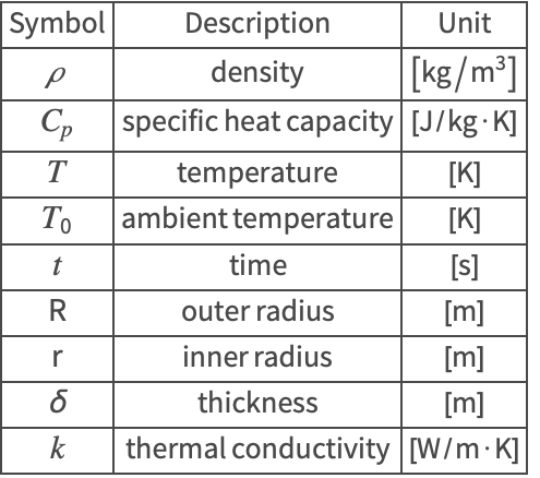
Nomenclature
References
1. Adamowicz, A. (2015). Axisymmetric FE model to analysis of thermal stresses in a brake disk. Journal of Theoretical and Applied Mechanics (Poland), 53(2), 409–420. https://doi.org/10.15632/jtam-pl.53.2.357