---
title: "BernoulliGraphDistribution"
language: "en"
type: "Symbol"
summary: "BernoulliGraphDistribution[n, p] represents a Bernoulli graph distribution for n-vertex graphs with edge probability p."
keywords: 
- Bernoulli random graph
- Binomial graph distribution
- Binomial random graph
- Poisson random graph
- Poisson graph
- Rapoport random graph
- Erdös random graph
- Erdös Renyi random graph
canonical_url: "https://reference.wolfram.com/language/ref/BernoulliGraphDistribution.html"
source: "Wolfram Language Documentation"
related_guides: 
  - 
    title: "Random Graphs"
    link: "https://reference.wolfram.com/language/guide/RandomGraphs.en.md"
  - 
    title: "Social Network Analysis"
    link: "https://reference.wolfram.com/language/guide/SocialNetworks.en.md"
  - 
    title: "Derived Statistical Distributions"
    link: "https://reference.wolfram.com/language/guide/DerivedDistributions.en.md"
related_functions: 
  - 
    title: "UniformGraphDistribution"
    link: "https://reference.wolfram.com/language/ref/UniformGraphDistribution.en.md"
  - 
    title: "BarabasiAlbertGraphDistribution"
    link: "https://reference.wolfram.com/language/ref/BarabasiAlbertGraphDistribution.en.md"
  - 
    title: "PriceGraphDistribution"
    link: "https://reference.wolfram.com/language/ref/PriceGraphDistribution.en.md"
  - 
    title: "DegreeGraphDistribution"
    link: "https://reference.wolfram.com/language/ref/DegreeGraphDistribution.en.md"
  - 
    title: "WattsStrogatzGraphDistribution"
    link: "https://reference.wolfram.com/language/ref/WattsStrogatzGraphDistribution.en.md"
  - 
    title: "BinomialDistribution"
    link: "https://reference.wolfram.com/language/ref/BinomialDistribution.en.md"
  - 
    title: "PoissonDistribution"
    link: "https://reference.wolfram.com/language/ref/PoissonDistribution.en.md"
---
# BernoulliGraphDistribution

BernoulliGraphDistribution[n, p] represents a Bernoulli graph distribution for n-vertex graphs with edge probability p.

## Details and Options

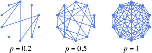
* The Bernoulli graph is constructed starting with the complete graph with ``n`` vertices and selecting each edge independently through a Bernoulli trial with probability ``p``.

* The following options can be given:

[`DirectedEdges`](https://reference.wolfram.com/language/ref/DirectedEdges.en.md) 	[`False`](https://reference.wolfram.com/language/ref/False.en.md)	whether to generate directed edges

* ``BernoulliGraphDistribution`` can be used with such functions as ``RandomGraph`` and ``GraphPropertyDistribution``.

---

## Examples (18)

### Basic Examples (2)

Generate a pseudorandom graph:

```wl
In[1]:= RandomGraph[BernoulliGraphDistribution[10, 0.6]]

Out[1]= [image]
```

---

Distribution of the number of edges:

```wl
In[1]:= \[ScriptCapitalD][n_, p_] = GraphPropertyDistribution[EdgeCount[g], g\[Distributed]BernoulliGraphDistribution[n, p]]

Out[1]= BinomialDistribution[(1/2) (-1 + n) n, p]
```

Probability density function:

```wl
In[2]:= PDF[\[ScriptCapitalD][n, p], m]

Out[2]=
Piecewise[{{(1 - p)^(-m + (1/2)*(-1 + n)*n)*p^m*Binomial[(1/2)*(-1 + n)*n, m], 
   0 <= m <= (1/2)*(-1 + n)*n}}, 0]

In[3]:= DiscretePlot[Evaluate @ Table[PDF[\[ScriptCapitalD][n, 1 / 2], m], {n, 3, 12, 3}], {m, 0, 50}, PlotRange -> All, ExtentSize -> 1 / 2]

Out[3]= [image]
```

### Scope (4)

Generate simple undirected graphs:

```wl
In[1]:= RandomGraph[BernoulliGraphDistribution[5, 0.6]]

Out[1]= [image]
```

---

Simple directed graphs:

```wl
In[1]:= RandomGraph[BernoulliGraphDistribution[5, 0.6, DirectedEdges -> True]]

Out[1]= [image]
```

---

Generate a set of pseudorandom graphs:

```wl
In[1]:= RandomGraph[BernoulliGraphDistribution[5, 0.8], 4]

Out[1]= {[image], [image], [image], [image]}
```

---

Compute probabilities and statistical properties:

```wl
In[1]:= \[ScriptCapitalD] = GraphPropertyDistribution[GlobalClusteringCoefficient[g], g\[Distributed]BernoulliGraphDistribution[5, 0.4]];

In[2]:= N[Mean[\[ScriptCapitalD]]]

Out[2]= 0.234702
```

### Options (2)

#### DirectedEdges (2)

By default, a Bernoulli graph is undirected:

```wl
In[1]:= RandomGraph[BernoulliGraphDistribution[10, 0.3]]

Out[1]= [image]

In[2]:= UndirectedGraphQ[%]

Out[2]= True
```

---

With the setting ``DirectedEdges -> True``, directed Bernoulli graphs are generated:

```wl
In[1]:= RandomGraph[BernoulliGraphDistribution[10, 0.3, DirectedEdges -> True]]

Out[1]= [image]

In[2]:= DirectedGraphQ[%]

Out[2]= True
```

### Applications (3)

After 20 children have spent their first week in kindergarten, the probability that two children have made friends is 0.2:

```wl
In[1]:= \[ScriptCapitalG] = BernoulliGraphDistribution[20, 0.2];

In[2]:= RandomGraph[\[ScriptCapitalG]]

Out[2]= [image]
```

Find the probability that the social network is connected:

```wl
In[3]:= NProbability[x == 1, x\[Distributed]GraphPropertyDistribution[Boole[ConnectedGraphQ[g]], g\[Distributed]\[ScriptCapitalG]]]

Out[3]= 0.745528
```

---

In a snowball fight with 15 participants, and everybody throwing snowballs at everyone else, the probability of being hit by any given participant is 0.4:

```wl
In[1]:= \[ScriptCapitalG] = BernoulliGraphDistribution[15, 0.4, DirectedEdges -> True];

In[2]:= RandomGraph[\[ScriptCapitalG]]

Out[2]= [image]
```

Find the size of the largest group where everybody has been hit by everyone else:

```wl
In[3]:= Length[First[FindClique[%]]]

Out[3]= 2
```

---

Find the largest component fraction when the mean vertex degree is $\beta$ :

```wl
In[1]:= \[ScriptCapitalD][n_, β_] := GraphPropertyDistribution[Length[First[ConnectedComponents[g]]] / n, g\[Distributed]BernoulliGraphDistribution[n, β / (n - 1)]]

In[2]:= Table[RandomVariate[\[ScriptCapitalD][10, β]], {β, 0, 3}]

Out[2]= {(1/10), 1, 1, 1}
```

Average the result over 100 runs and plot it for different numbers of vertices:

```wl
In[3]:= Table[Plot[Mean[RandomVariate[\[ScriptCapitalD][10, β], 100]], {β, 0, 3}, MaxRecursion -> 2, PlotLabel -> n], {n, {10, 100}}]

Out[3]= {[image], [image]}
```

### Properties & Relations (6)

Distribution of the number of vertices:

```wl
In[1]:= GraphPropertyDistribution[VertexCount[g], g\[Distributed]BernoulliGraphDistribution[n, p]]

Out[1]= DiscreteUniformDistribution[{n, n}]
```

---

Distribution of the number of edges:

```wl
In[1]:= \[ScriptCapitalD][n_, p_] = GraphPropertyDistribution[EdgeCount[g], g\[Distributed]BernoulliGraphDistribution[n, p]]

Out[1]= BinomialDistribution[(1/2) (-1 + n) n, p]
```

Probability density function:

```wl
In[2]:= PDF[\[ScriptCapitalD][n, p], m]

Out[2]=
Piecewise[{{(1 - p)^(-m + (1/2)*(-1 + n)*n)*p^m*Binomial[(1/2)*(-1 + n)*n, m], 
   0 <= m <= (1/2)*(-1 + n)*n}}, 0]

In[3]:= DiscretePlot[Evaluate @ Table[PDF[\[ScriptCapitalD][n, 0.4], x], {n, 3, 12, 3}], {x, 0, 40}, PlotRange -> All, ExtentSize -> 1 / 2]

Out[3]= [image]
```

The mean of the number of edges:

```wl
In[4]:= Mean[\[ScriptCapitalD][n, p]]

Out[4]= (1/2) (-1 + n) n p
```

---

Distribution of the degree of a vertex:

```wl
In[1]:= \[ScriptCapitalD][n_, p_] = GraphPropertyDistribution[VertexDegree[g, v], g\[Distributed]BernoulliGraphDistribution[n, p]]

Out[1]= BinomialDistribution[-1 + n, p]
```

Probability density function:

```wl
In[2]:= PDF[\[ScriptCapitalD][n, p], k]

Out[2]= Piecewise[{{(1 - p)^(-1 - k + n)*p^k*Binomial[-1 + n, k], 0 <= k <= -1 + n}}, 0]

In[3]:= DiscretePlot[Evaluate @ Table[PDF[\[ScriptCapitalD][n, 0.3], x], {n, 5, 50, 15}], {x, 0, 25}, PlotRange -> All, ExtentSize -> 1 / 2]

Out[3]= [image]
```

The mean of the degree of a vertex:

```wl
In[4]:= Mean[\[ScriptCapitalD][n, p]]

Out[4]= (-1 + n) p
```

---

Connectivity for large ``n`` with respect to ``p`` :

```wl
In[1]:= \[ScriptCapitalD][n_, p_] := GraphPropertyDistribution[Boole[ConnectedGraphQ[g]], g\[Distributed]BernoulliGraphDistribution[n, p]]
```

A Bernoulli graph is almost surely disconnected for $n p<\log (n)$ :

```wl
In[2]:= NProbability[x == 0, x\[Distributed]\[ScriptCapitalD][500, 0.01], Method -> {"MonteCarlo", PrecisionGoal -> 1}]

Out[2]= 0.964
```

A Bernoulli graph is almost surely connected for $n p>\log (n)$ :

```wl
In[3]:= NProbability[x == 1, x\[Distributed]\[ScriptCapitalD][500, 0.02], Method -> {"MonteCarlo", PrecisionGoal -> 1}]

Out[3]= 0.9785
```

---

Use ``BernoulliDistribution`` to simulate a ``BernoulliGraphDistribution`` :

```wl
In[1]:=
bernoulli[n_, p_] := 
	Graph[Range[n], Pick[EdgeList[CompleteGraph[n]], 
	RandomVariate[BernoulliDistribution[p], n(n - 1) / 2], 1]]
```

Pseudorandom graphs:

```wl
In[2]:= Table[bernoulli[10, p], {p, 0.3, 1, 0.2}]

Out[2]= {[image], [image], [image], [image]}
```

---

Edge probability 1 results in the ``CompleteGraph`` :

```wl
In[1]:= RandomGraph[BernoulliGraphDistribution[5, 1]]

Out[1]= [image]

In[2]:= CompleteGraphQ[%]

Out[2]= True
```

Edge probability 0 results in the empty graph:

```wl
In[3]:= RandomGraph[BernoulliGraphDistribution[5, 0]]

Out[3]= [image]

In[4]:= EmptyGraphQ[%]

Out[4]= True
```

### Neat Examples (1)

Randomly colored vertices:

```wl
In[1]:= HighlightGraph[RandomGraph[BernoulliGraphDistribution[10 ^ 2, 0.03]], Table[Style[i, RandomChoice[ColorData[45, "ColorList"]]], {i, 10 ^ 2}]]

Out[1]= [image]
```

## See Also

* [`UniformGraphDistribution`](https://reference.wolfram.com/language/ref/UniformGraphDistribution.en.md)
* [`BarabasiAlbertGraphDistribution`](https://reference.wolfram.com/language/ref/BarabasiAlbertGraphDistribution.en.md)
* [`PriceGraphDistribution`](https://reference.wolfram.com/language/ref/PriceGraphDistribution.en.md)
* [`DegreeGraphDistribution`](https://reference.wolfram.com/language/ref/DegreeGraphDistribution.en.md)
* [`WattsStrogatzGraphDistribution`](https://reference.wolfram.com/language/ref/WattsStrogatzGraphDistribution.en.md)
* [`BinomialDistribution`](https://reference.wolfram.com/language/ref/BinomialDistribution.en.md)
* [`PoissonDistribution`](https://reference.wolfram.com/language/ref/PoissonDistribution.en.md)

## Related Guides

* [Random Graphs](https://reference.wolfram.com/language/guide/RandomGraphs.en.md)
* [Social Network Analysis](https://reference.wolfram.com/language/guide/SocialNetworks.en.md)
* [Derived Statistical Distributions](https://reference.wolfram.com/language/guide/DerivedDistributions.en.md)

## History

* [Introduced in 2010 (8.0)](https://reference.wolfram.com/language/guide/SummaryOfNewFeaturesIn80.en.md)