

DiscreteAsymptotic
DiscreteAsymptotic[expr,n∞]
gives an asymptotic approximation for expr as n tends to infinity over the integers.
DiscreteAsymptotic[expr,{n,∞,m}]
gives an asymptotic series approximation for expr to order m.
Details and Options
- DiscreteAsymptotic is typically used to solve problems for which no exact solution can be found or to get simpler answers for computation, comparison and interpretation. In such cases, an asymptotic approximation often gives enough information for simplifying or solving application problems.
- DiscreteAsymptotic[expr,n∞] computes the leading term in an asymptotic expansion for expr. Use SeriesTermGoal to specify more terms.
- The expression expr can be any sequence
 , a sum specified by Sum, a product specified by Product, a sequence specified by SeriesCoefficient, a difference equation specified by RSolveValue, etc.
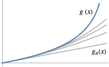
 - If the exact result is g[x] and the asymptotic approximation of order n at x0 is gn[x], then AsymptoticLess[g[x]-gn[x],gn[x]-gn-1[x],xx0] or g[x]-gn[x]∈o[gn[x]-gn-1[x]] as xx0.
- The asymptotic approximation gn[x] is often given as a sum gn[x]
 αkϕk[x], where {ϕ1[x],…,ϕn[x]} is an asymptotic scale ϕ1[x]≻ϕ2[x]≻⋯>ϕn[x] as xx0. Then AsymptoticLess[g[x]-gn[x],ϕn[x],xx0] or g[x]-gn[x]∈o[ϕn[x]] as xx0.
 - Common asymptotic scales include:
-

Taylor scale when xx0 
Laurent scale when xx0 
Laurent scale when x±∞ 
Puiseux scale when xx0 - The scales used to express the asymptotic approximation are automatically inferred from the problem and can often include more exotic scales.
- The following options can be given:
-
AccuracyGoal Automatic digits of absolute accuracy sought Assumptions $Assumptions assumptions to make about parameters GenerateConditions Automatic whether to generate answers that involve conditions on parameters GeneratedParameters None how to name generated parameters Method Automatic method to use PerformanceGoal $PerformanceGoal aspects of performance to optimize PrecisionGoal Automatic digits of precision sought SeriesTermGoal Automatic number of terms in the approximation WorkingPrecision Automatic the precision used in internal computations - With the default setting of Automatic for GenerateConditions, conditions on parameters are typically not returned in the results from DiscreteAsymptotic. Answers that include conditions on parameters may be obtained by setting GenerateConditions to True.
- Possible settings for PerformanceGoal include $PerformanceGoal, "Quality" and "Speed". With the "Quality" setting, DiscreteAsymptotic typically solves more problems or produces simpler results, but it potentially uses more time and memory.
- With the default setting of Automatic for WorkingPrecision, AccuracyGoal and PrecisionGoal, DiscreteAsymptotic may return an asymptotic approximation with a lower precision, even if the input has infinite precision.
Examples
open all close allBasic Examples (4)
Find the leading asymptotic term for ![]() as
as ![]() approaches Infinity:
approaches Infinity:
DiscreteAsymptotic[n!, n -> ∞]Compare the values of the sequence, the approximation and their ratios:
Table[{n!, N[%], n! / N[%]}, {n, 1, 21, 4}]//TableFormUse SeriesTermGoal to obtain more terms from the expansion:
DiscreteAsymptotic[n!, n -> ∞, SeriesTermGoal -> 3]Find the asymptotic behavior of a sequence using its generating function:
genfun = (1/2 - E^z);Apply DiscreteAsymptotic to compute an asymptotic approximation:
asy = DiscreteAsymptotic[SeriesCoefficient[genfun, {z, 0, n}], n -> ∞]Table[asy, {n, 0, 20, 5}]//NCompare the approximation with the values of the sequence:
Table[SeriesCoefficient[genfun, {z, 0, n}], {n, 0, 20, 5}]//NCompute an asymptotic approximation for a definite sum:
DiscreteAsymptotic[Inactive[Sum][Binomial[n, k] ^ 2, {k, 0, n}], n -> ∞]Obtain the same result using AsymptoticSum:
AsymptoticSum[Binomial[n, k] ^ 2, {k, 0, n}, n -> ∞]Compute an asymptotic approximation for a difference equation:
dr = DifferenceRoot[Function[{y, n}, {y[n + 1] - n ^ 2 y[n] == 0, y[1] == 1}]][n];DiscreteAsymptotic[dr, n -> ∞]Obtain the same result using AsymptoticRSolveValue:
AsymptoticRSolveValue[{y[n + 1] - n ^ 2 * y[n] == 0, y[1] == 1}, y[n], n -> ∞]Scope (19)
Elementary Sequences (8)
Leading asymptotic term for a polynomial sequence:
DiscreteAsymptotic[n ^ 4 + 5n ^ 3 + 3n - 11, n -> ∞]Plot the sequence and the approximation:
DiscretePlot[{n ^ 4 + 5n ^ 3 + 3n - 11, n ^ 4}, {n, 1, 20}]DiscreteAsymptotic[(3n ^ 2 + 5) / (4n ^ 2 + 11), n -> ∞]DiscreteAsymptotic[(3n ^ 3 + 5) / (4n ^ 2 + 11), n -> ∞]DiscreteAsymptotic[(3n + 5) / (4n ^ 2 + 11), n -> ∞]DiscreteAsymptotic[2 ^ n, n -> ∞]DiscreteAsymptotic[2 ^ n + 3 ^ (-n), n -> ∞]Polynomial exponential sequences:
DiscreteAsymptotic[n ^ 2 2 ^ n, n -> ∞]DiscreteAsymptotic[(n ^ 2 + 3n)2 ^ n, n -> ∞]Rational exponential sequences:
DiscreteAsymptotic[(n ^ 2 / (3n ^ 2 + 1))2 ^ n, n -> ∞]DiscreteAsymptotic[(n ^ 2 / (3n ^ 3 + 1))2 ^ n, n -> ∞]DiscreteAsymptotic[(5n ^ 4 / (3n ^ 3 + 1))2 ^ n, n -> ∞]DiscreteAsymptotic[Sinh[n], n -> ∞]DiscreteAsymptotic[ArcSinh[n], n -> ∞]DiscreteAsymptotic[Log[n], n -> ∞]DiscreteAsymptotic[(5n ^ 2 / (3n ^ 3 + 1))Log[n], n -> ∞]DiscreteAsymptotic[(5n ^ 4 / (3n ^ 3 + 1))Log[n], n -> ∞]DiscreteAsymptotic[2 ^ n / (1 + 2 ^ n), n -> ∞]DiscreteAsymptotic[4 ^ n / (1 + 2 ^ n), n -> ∞]DiscreteAsymptotic[2 ^ n / (1 + 4 ^ n), n -> ∞]DiscreteAsymptotic[QPolyGamma[2, n], n -> ∞]Special Sequences (6)
Find the leading asymptotic term for Fibonacci as ![]() approaches Infinity:
approaches Infinity:
DiscreteAsymptotic[Fibonacci[n], n -> ∞]Compare the sequence and the approximation:
Table[{Fibonacci[n], N[%]}, {n, 1, 21, 4}]//TableFormLeading asymptotic term for Pochhammer:
DiscreteAsymptotic[Pochhammer[a, n], n -> ∞]DiscreteAsymptotic[FactorialPower[a, n], n -> ∞]DiscreteAsymptotic[Binomial[n, k], n -> ∞]Leading asymptotic term for HarmonicNumber:
DiscreteAsymptotic[HarmonicNumber[n], n -> ∞]DiscreteAsymptotic[PolyGamma[n], n -> ∞]Zeta:
DiscreteAsymptotic[Zeta[n], n -> ∞]Leading asymptotic term for StirlingS1:
DiscreteAsymptotic[StirlingS1[n, 2], n -> ∞]DiscreteAsymptotic[StirlingS2[n, 2], n -> ∞]Compare with the exact value for ![]() :
:
% /. {n -> 200.`20}//NStirlingS2[200, 2]//NLeading asymptotic term for BellB:
DiscreteAsymptotic[BellB[n], n -> ∞]Compare with the exact value for ![]() :
:
% /. {n -> 1400.`20}//NBellB[1400]//NLeading asymptotic term for BernoulliB:
DiscreteAsymptotic[BernoulliB[2n], n -> ∞]DiscreteAsymptotic[EulerE[2n], n -> ∞]Sums and Summation Transforms (3)
Compute an asymptotic approximation for a definite sum:
DiscreteAsymptotic[Inactive[Sum][1 / (k ^ 2 + a), {k, 0, Infinity}], a -> 0]Obtain the same result using AsymptoticSum:
AsymptoticSum[1 / (k ^ 2 + a), {k, 0, Infinity}, a -> 0]Compute an asymptotic approximation for the Fibonacci sequence using its generating function:
DiscreteAsymptotic[Inactive[SeriesCoefficient][-(z / (-1 + z + z ^ 2)), {z, 0, n}],
n -> ∞]% /. {n -> 2000.}Fibonacci[2000]//NCompute a leading asymptotic approximation for an inverse Z transform:
DiscreteAsymptotic[Inactive[InverseZTransform][1 / (z * (-6 + 6 * z ^ 2 + z ^ 3)), z, n], n -> ∞]Difference Equations (2)
Compute an asymptotic approximation for a first-order difference equation:
dr = DifferenceRoot[Function[{, }, {-(n * []) + [1 + ] == 0, [1] == 1}]][n];DiscreteAsymptotic[dr, n -> Infinity]Obtain the same result using AsymptoticRSolveValue:
AsymptoticRSolveValue[{y[n + 1] - n * y[n] == 0, y[1] == 1}, y[n], n -> ∞]Compute an asymptotic approximation for a higher-order difference equation:
DiscreteAsymptotic[Inactive[RSolveValue][{n ^ 4y[n + 2] == 2n ^ 3(n - 1) y[n + 1] - (n ^ 4 - 2n ^ 3 - 1)y[n], y[1] == 1., y[2] == 3}, y[n], n],
n -> ∞, SeriesTermGoal -> 7]
Options (1)
SeriesTermGoal (1)
By default, DiscreteAsymptotic returns the leading term in the asymptotic expansion:
DiscreteAsymptotic[n!, n -> ∞]DiscreteAsymptotic[n!, n -> ∞, SeriesTermGoal -> 1]Use SeriesTermGoal to obtain more terms from the expansion:
DiscreteAsymptotic[n!, n -> ∞, SeriesTermGoal -> 3]Obtain the same result using a list specification:
DiscreteAsymptotic[n!, {n, ∞, 3}]Applications (3)
Find the leading asymptotic term for Prime as ![]() approaches Infinity:
approaches Infinity:
DiscreteAsymptotic[Prime[n], n -> ∞]Plot the sequence and the approximation:
DiscretePlot[{Prime[n], %}, {n, 100, 1000, 10}, PlotLegends -> {Prime[n], n Log[n]}]Compare the numerical values of the sequence and its approximation:
{Prime[1000], 1000 Log[1000.]}The ratio of the sequence and its leading asymptotic approaches 1 as ![]() approaches Infinity:
approaches Infinity:
DiscreteLimit[Prime[n] / (n Log[n]), n -> ∞]Compute an asymptotic approximation for a binomial sum:
DiscreteAsymptotic[Sum[Binomial[n, k] ^ 3, {k, 0., n}], n -> ∞]Compare the approximate and exact values for ![]() :
:
% /. {n -> 1000.}Sum[Binomial[1000, k] ^ 3, {k, 0, 1000}]//NCompute the leading-order asymptotic term for the Apéry sequence, which satisfies the following linear second-order difference equation:
apeqn = (n + 2) ^ 3 u[n + 2] - (34 n ^ 3 + 153 n ^ 2 + 231 n + 117)u[n + 1] + (n + 1) ^ 3 u[n] == 0;Obtain the leading asymptotic term:
sol[n_] = DiscreteAsymptotic[Inactive[RSolveValue][apeqn, u[n], n], n -> Infinity]Assign a value to ![]() based on the defining sum for the sequence:
based on the defining sum for the sequence:
tsol[n_] := Sum[Binomial[n, k] ^ 2 Binomial[n + k, k] ^ 2, {k, 0, n}]Solve[sol[1000] == tsol[1000], C[2]]//N[#, 20]&//ChopObtain an approximate value for a member of the sequence:
sol[10000] /. %[[1]] //N[#, 20]&Compare with the corresponding Apéry number:
tsol[10000]//NProperties & Relations (2)
The result from DiscreteAsymptotic is asymptotically equivalent to the sequence:
DiscreteAsymptotic[(n ^ 2 + 3) / (5n ^ 3 + 11), n -> ∞]Use AsymptoticEquivalent to verify the result:
AsymptoticEquivalent[(n ^ 2 + 3) / (5n ^ 3 + 11), 1 / (5n), n -> ∞]DiscreteAsymptotic describes the behavior of a sequence for large values of ![]() :
:
DiscreteAsymptotic[2 ^ n / (1 + 4 ^ n), n -> ∞]% /. {n -> 500.}DiscreteLimit describes the behavior of the sequence at Infinity:
DiscreteLimit[2 ^ n / (1 + 4 ^ n), n -> ∞]Text
Wolfram Research (2020), DiscreteAsymptotic, Wolfram Language function, https://reference.wolfram.com/language/ref/DiscreteAsymptotic.html.
CMS
Wolfram Language. 2020. "DiscreteAsymptotic." Wolfram Language & System Documentation Center. Wolfram Research. https://reference.wolfram.com/language/ref/DiscreteAsymptotic.html.
APA
Wolfram Language. (2020). DiscreteAsymptotic. Wolfram Language & System Documentation Center. Retrieved from https://reference.wolfram.com/language/ref/DiscreteAsymptotic.html