ItoProcess[{a,b},x,t]
表示伊藤 (Ito) 过程  ,其中
,其中  .
.
ItoProcess[{a,b,c},x,t]
表示伊藤过程  ,其中
,其中  .
.
ItoProcess[…,{x,x0},{t,t0}]
使用初始条件 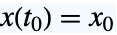 .
.
ItoProcess[…,…,…,Σ]
使用维纳过程  ,其中协方差为 Σ.

ItoProcess
ItoProcess[{a,b},x,t]
表示伊藤 (Ito) 过程  ,其中
,其中  .
.
ItoProcess[{a,b,c},x,t]
表示伊藤过程  ,其中
,其中  .
.
ItoProcess[…,{x,x0},{t,t0}]
使用初始条件 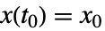 .
.
ItoProcess[…,…,…,Σ]
使用维纳过程  ,其中协方差为 Σ.
ItoProcess[proc]
在可能的情况下,将 proc 转化为标准伊藤过程.
ItoProcess[sdeqns,expr,x,t,wdproc]
表示由随机微分方程 sdeqns、输出表达式 expr 指定的伊藤过程,其中状态为 x,时间为 t,由遵循过程 dproc 的 w 驱动.
更多信息和选项
- ItoProcess 也称为 Ito 扩散或者随机微分方程 (SDE).
- ItoProcess 是连续时间和连续状态随机过程.
- 如果 drift a 是
 维向量,而扩散率 b 为
  ×
× 维矩阵,过程
  是维的,并且由
  维 WienerProcess 驱动.
 - 系数 a 和 b 的常见指定包括:
-
a 标量,b 标量 
a 标量,b 向量 
a 向量,b 向量 
a 向量,b 矩阵 
- 随机微分方程
 有时候写作积分方程
  .
. - 默认初始时间 t0 为零,而默认初始状态 x0 为零.
- 默认协方差 Σ 是恒等矩阵.
- 对于广义协方差 Σ,通过将扩散矩阵 b 转换成 b.Σ1/2(其中,可能的情况下, Σ1/2 为 Σ 的下 Cholesky 因子),ItoProcess 将过程标准化. »
- 标准伊藤过程具有输出
 ,包括微分状态
  的子集.
的子集. - 可被转化为标准 ItoProcess 格式的过程 proc 包括 OrnsteinUhlenbeckProcess、 GeometricBrownianMotionProcess、StratonovichProcess 和 ItoProcess.
- 将 ItoProcess 转化为标准格式自动利用伊藤引理.
- sdeqns 中的随机微分方程的格式是
 ,其中
,其中  是 \[DifferentialD],它可以使用
  dd
dd 输入. 导数
  和
和  为伊藤导数.
 - 输出表达式 expr 可以涉及 x[t] 和 t 的任何表达式.
- 驱动过程 dproc 可以是任何可被转化为标准伊藤过程.
- 与 ItoProcess 相关的属性包括:
-
"Drift" 漂移项 "Diffusion" 扩散矩阵 "Output" 输出状态 "TimeVariable" 时间变量 "TimeOrigin" 时间变量原点 "StateVariables" 状态变量 "InitialState" 初始状态值 "KolmogorovForwardEquation" 柯尔莫哥洛夫 (Kolmogorov) 前向方程 (福克-普朗克 (Fokker-Planck) 方程) "KolmogorovBackwardEquation" 柯尔莫哥洛夫后向方程 "Derivative" 伊藤 (Ito) 导数 "FeynmanKacFormula" 从 Feynman-Kac 公式中得到的偏微分方程 (PDE) - RandomFunction 中 ItoProcess 特定的 Method 设置包括: »
-
"EulerMaruyama" Euler–Maruyama(阶数为 1/2,默认) "KloedenPlatenSchurz" Kloeden–Platen–Schurz(阶数为3/2) "Milstein" Milstein(阶数为 1) "StochasticRungeKutta" 3‐阶段 Rossler SRK 方案(阶数为 1) "StochasticRungeKuttaScalarNoise" 标量噪声的 3‐阶段 Rossler SRK 方案(阶数为3/2) - ItoProcess 可以与诸如 RandomFunction、CovarianceFunction、PDF 和 Expectation 等函数一起使用.
范例
打开所有单元 关闭所有单元基本范例 (1)
proc = ItoProcess[ⅆx[t] == -x[t]ⅆt + Sqrt[1 + x[t] ^ 2]ⅆw[t], x[t], {x, 1}, t, wWienerProcess[]]RandomFunction[proc, {0., 5., 0.01}]ListLinePlot[%, Filling -> Axis]Mean[proc[t]]CovarianceFunction[proc, s, t]Plot3D[%, {s, 0, 5}, {t, 0, 5}, ColorFunction -> "Rainbow"]范围 (19)
基本用途 (10)
从随机微分方程(SDE) 定义 Wiener 过程,其中 drift 为
  和扩散率为
和扩散率为  :
:
ItoProcess[{μ, σ}, {x, 0}, t]ItoProcess[WienerProcess[μ, σ]]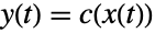

ItoProcess[{μ, σ, c[x[t]]}, {x, 0}, t]ItoProcess[ⅆx[t] == μ ⅆt + σ ⅆw[t], c[x[t]], {x, 0}, t, wWienerProcess[]]

ItoProcess[{{v, -x}, {0, 1}, x}, {{x, v}, {x0, v0}}, {t, 0}]ItoProcess[{ⅆx[t] == v[t] ⅆt, ⅆv[t] == -x[t]ⅆt + ⅆw[t]}, x[t], {{x, v}, {x0, v0}}, t, wWienerProcess[]]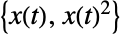

ItoProcess[{μ, σ, {x, x ^ 2}}, {x, 0}, t]ItoProcess[ⅆx[t] == μⅆt + σ ⅆw[t], {x[t], x[t] ^ 2}, {x, 0}, t, wWienerProcess[]]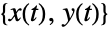

ItoProcess[{{y, -x}, {{1, 0}, {0, 1}}}, {{x, y}, {0, 0}}, t]ItoProcess[{ⅆx[t] == y[t]ⅆt + ⅆw1[t], ⅆy[t] == -x[t]ⅆt + ⅆw2[t]}, {x[t], y[t]}, {{x, y}, {0, 0}}, t, {w1WienerProcess[], w2WienerProcess[]}]Σ = {{1, 3 / 5}, {3 / 5, 1}};b = {{Subscript[σ, 1], Subscript[σ, 2]}};
proc = ItoProcess[{{1 - x[t]}, b, x[t]}, {{x}, {1 / 2}}, {t, 0}, Σ]规范化过程具有等于  的扩散矩阵,其中
  是规范化前的扩散矩阵:
bnew = proc[[1, 2]]bnew == b.CholeskyDecomposition[Σ]

ItoProcess[ⅆx[t] == Subscript[w, 1][t]ⅆSubscript[w, 2][t], x[t], {x, 0}, t, {Subscript[w, 1]WienerProcess[], Subscript[w, 2]WienerProcess[]}]



ItoProcess[{ⅆx[t] == Subscript[w, 1][t]ⅆSubscript[w, 2][t], ⅆy[t] == Subscript[w, 1][t]ⅆSubscript[w, 1][t]}, {x[t], y[t]}, {{x, y}, {0, 0}}, t, {Subscript[w, 1]WienerProcess[], Subscript[w, 2]WienerProcess[]}]noise𝒫[σ1_, σ2_, ρ_] = Refine[ItoProcess[{{0, 0}, {{σ1, 0}, {0, σ2}}}, {{w1, w2}, {0, 0}}, t, {{1, ρ}, {ρ, 1}}], -1 < ρ < 1];ItoProcess[{ⅆs[t] == μ s[t]ⅆt + Sqrt[r[t]]s[t]ⅆn1[t], ⅆr[t] == θ(μ - r[t])ⅆt + Sqrt[r[t]]ⅆn2[t]
}, {s[t], r[t]}, {{s, r}, {s0, r0}}, t, {n1, n2}noise𝒫[Subscript[σ, 1], Subscript[σ, 2], ρ]]用不同的方法模拟 ItoProcess 的路径:
proc = ItoProcess[{ⅆx[t] == v[t]ⅆt, ⅆv[t] == -x[t]ⅆt + ⅆn[t]}, x[t], {{x, v}, {1, 0}}, t, nWienerProcess[]]methods = {"EulerMaruyama", "Milstein", "StochasticRungeKutta", "KloedenPlatenSchurz", "StochasticRungeKuttaScalarNoise"};orders = {"order 1/2", "order 1", "order 1", "order 3/2", "order 3/2"};用 RandomFunction 中的选项指定模拟方法:
paths = Table[RandomFunction[proc, {0., 2. Pi, 0.05}, 6, Method -> m], {m, methods}];Grid[Partition[MapThread[ListLinePlot[#1, PlotLabel -> Column[{#2, #3}], ImageSize -> 160]& , {paths, methods, orders}], UpTo[3]], Spacings -> 2]过程属性提取 (2)
proc = ItoProcess[ⅆx[t] == (μ - x[t])ⅆt + Sqrt[1 + x[t] ^ 2]ⅆw[t], x[t], {x, 1}, t, wWienerProcess[]]proc["Properties"]proc /@ {"Drift", "Diffusion"}proc["KolmogorovForwardEquation"]//TraditionalForm此处使用 Inactive 来避免扩展偏导数;使用 Activate 来扩展表达式:
Activate[%]//TraditionalFormproc["KolmogorovBackwardEquation"]//TraditionalForm计算函数  的伊藤导数. 输出是一个由漂移和扩散项组成的列表:
{mu, sig} = proc["Derivative", f[x[t], t]];TraditionalForm[mu]TraditionalForm[sig]属性 "FeynmanKacFormula" 给出了一个偏微分方程,其解  满足条件期望
  和终止条件
和终止条件  :
:
proc["FeynmanKacFormula"]//TraditionalForm对于广义情况,可以提供额外的论据. 有了额外的参数  后,"FeynmanKacFormula" 属性可给出一个偏微分方程,其解决方案满足条件期望
  和相同的终止条件:
proc["FeynmanKacFormula", α[x, t]]//TraditionalForm使用第三个参数  ,属性 "FeynmanKacFormula" 会给出偏微分方程,其解满足条件期望
  和相同的终止条件:
proc["FeynmanKacFormula", α[x, t], β[x, t]]//TraditionalForm使用 ItoProcess 定义 Heston 模型:
heston = ItoProcess[{{μ S[t], κ(θ - ν[t])}, {{ν[t]^1 / 2S[t], 0}, {0, σ ν[t]^1 / 2}}}, {{S, ν}, {Subscript[S, 0], Subscript[ν, 0]}}, t, {{1, 1 / 2}, {1 / 2, 1}}]heston["Drift"]heston["Diffusion"]heston["KolmogorovForwardEquation"]//TraditionalFormheston["KolmogorovBackwardEquation"]//TraditionalForm{mu, sig} = heston["Derivative", f[S[t], ν[t], t]];mu//TraditionalFormsig//TraditionalForm特殊 Ito 过程 (5)
对应于 WienerProcess 的伊藤过程:
ItoProcess[WienerProcess[μ, σ]]对应于 GeometricBrownianMotionProcess 的伊藤过程:
ItoProcess[GeometricBrownianMotionProcess[μ, σ, x0]]对应于 BrownianBridgeProcess 的伊藤过程:
ItoProcess[BrownianBridgeProcess[σ, {Subscript[t, 1], a}, {Subscript[t, 2], b}]]对应于 OrnsteinUhlenbeckProcess 的伊藤过程:
ItoProcess[OrnsteinUhlenbeckProcess[μ, σ, θ, x0]]对应于 CoxIngersollRossProcess 的伊藤过程:
ItoProcess[CoxIngersollRossProcess[μ, σ, θ, x0]]过程切片属性 (2)
Jacobi𝒫[x0_] := ItoProcess[ⅆx[t] == (1 / 2 - x[t])ⅆt + Sqrt[x[t](1 - x[t])]ⅆw[t], x[t], {x, x0}, t, wWienerProcess[]]Table[Cumulant[Jacobi𝒫[x0][t], r], {r, 1, 4}]Limit[%, t -> ∞]Table[Cumulant[UniformDistribution[], r], {r, 1, 4}]proc[{σ1_, σ2_}, {x0_, y0_}] = ItoProcess[ⅆx[t] == -(x[t] + y[t])ⅆt + σ1 ⅆw[t] && ⅆy[t] == -2x[t]ⅆt + σ2ⅆw[t], {x[t], y[t]}, {{x, y}, {x0, y0}}, t, wWienerProcess[]]PDF[proc[{1, -1}, {1 / 2, -1 / 4}][t], {x, y}]

cov = Covariance[proc[{Subscript[σ, 1], Subscript[σ, 2]}, {x0, y0}][t], 1, 2]
Collect[cov, E ^ _, Simplify]应用 (11)
计算属性 (3)
计算 Ornstein‐Uhlenbeck 过程  的交叉协方差和它的内在 Wiener 过程
  :
:
joint𝒫 = ItoProcess[ⅆx[t] == θ(μ - x[t])ⅆt + σ ⅆw[t], {x[t], w[t]}, {x, x0}, t, wWienerProcess[]]Covariance[joint𝒫[t], 1, 2]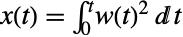

ItoProcess[ⅆx[t] == w[t] ^ 2ⅆt, x[t], {x, 0}, t, wWienerProcess[]]Table[Moment[%[t], r], {r, 0, 8}]proc = ItoProcess[{ⅆx[t] == v[t]ⅆt, ⅆv[t] == -x[t]ⅆt + ⅆn[t]}, x[t], {{x, v}, {1, 0}}, t, nWienerProcess[]]path = RandomFunction[proc, {0., 2. Pi, 0.05}, 12, Method -> "StochasticRungeKutta"];ListLinePlot[path]mf[t_] = Mean[proc[t]]vf[t_] = Simplify[Variance[proc[t]]]Show[Plot[{mf[t] - Sqrt[vf[t]], mf[t] + Sqrt[vf[t]], mf[t]}, {t, 0, 2Pi}, Filling -> {1 -> {2}}], ListLinePlot[path], PlotRange -> All]鞅 (Martingales) (3)
确定  和
和  的值,以满足过程
  是 martingale,其中
  是标准 Wiener 过程:
x𝒫 = ItoProcess[{0, 1, Exp[α w[t] + β t]}, {w, 0}, t]st𝒫 = ItoProcess[x𝒫]
Reduce[st𝒫[[1, 1]] == 0, {α, β}]ItoProcess[{0, {1, 1, 1}}, {x, 0}, {t, 0}]ItoProcess[ⅆx[t] == ⅆw1[t] + ⅆw2[t] + ⅆw3[t], x[t], {x, 0}, t, {w1WienerProcess[], w2WienerProcess[], w3WienerProcess[]}]proc1 = ItoProcess[ⅆx[t] == (w1[t]/Sqrt[w1[t]^2 + w2[t]^2])ⅆw1[t] + (w2[t]/Sqrt[w1[t]^2 + w2[t]^2])ⅆw2[t], x[t], {x, x0}, t, {w1WienerProcess[], w2WienerProcess[]}]
Integrate[Simplify[#.#&[proc1["Derivative", x[t]][[2, 1]]]], {t, 0, t}]通过列维 (Lévy) 表征, 是布朗运动. 该过程的均值与初始状态相同:
Mean[proc1[t]]建模 (2)
自由粒子在热涨落作用下的动力学可以用朗之万运动方程建模, ,其中
,其中  是标准的 WienerProcess,
 是热噪声的强度. 这里假设
  只能取决于
只能取决于  并专注于速度方程. 积分运动方程的常用方法有两种:伊藤公式和斯特拉托诺维奇公式. 可以通过以下方式定义:
ito = ItoProcess[ⅆv[t] == -v[t]ⅆt + σ[v[t]]ⅆb[t], v[t], {v, vi}, t, bWienerProcess[]];str = StratonovichProcess[ⅆv[t] == -v[t]ⅆt + σ[v[t]]ⅆb[t], v[t], {v, vs}, t, bWienerProcess[]];当  为常数时,这两个公式是相同的,并导致当
  时相同的平稳分布:
Limit[PDF[ito[t] /. {σ[v[t]] -> Sqrt[2]σ1}, v]//Simplify, t -> Infinity]Limit[PDF[str[t] /. {σ[v[t]] -> Sqrt[2]σ1}, v]//Simplify, t -> Infinity]如果  与速度有关,则由于 WienerProcess 的性质,
 具有非零二次变化,且两个公式会导致不同的结果. 将斯特拉托诺维奇公式转换为等效的伊藤公式:
istr = ItoProcess[str]ito["Drift"]istr["Drift"]Gompertz 曲线通常被用于模拟生长过程,比如肿瘤的生长. 通过假设生长过程的对数中的高斯噪声,可以把模型写成随机微分方程:
proc = ItoProcess[ⅆX[t] == -α Exp[-α t]Log[X0 / K]X[t]ⅆt + σ X[t]ⅆW[t], X[t], {X, X0}, t, WWienerProcess[]]Mean[proc[t]]过程在时间  的切片分布服从 LogNormalDistribution:
PDF[proc[t], x]


proc1 = proc /. {X0 -> 1, K -> 2, σ -> 0.1, α -> 0.3};sample = RandomFunction[proc1, {0, 10, 0.01}];ListLinePlot[sample, Filling -> Axis]产生同样条件下的一千个样本,然后可视化路径并在  对数据进行切片:
samples = RandomFunction[proc1, {0, 10, 0.1}, 1000];GraphicsRow[{ListLinePlot[samples, ImageSize -> 250, PlotRange -> All,
AspectRatio -> 3 / 4, BaseStyle -> Directive[Thin, Opacity[0.5]], PlotRangePadding -> {{0, .25}, {.5, .5}}], Histogram[samples["SliceData", 10], Automatic, "PDF"]}]伊藤过程表示 (3)
使用 ItoProcess 来表示标准 WienerProcess:
wiener = ItoProcess[ⅆB[t] == ⅆw[t], B[t], {B, 0}, t, wWienerProcess[]]

M = Exp[t / 2]Sin[B[t]];
{drift, diffusion} = wiener["Derivative", M]
创建一个 CoxIngersollRossProcess 并使用 ItoProcess 表示:
cir = CoxIngersollRossProcess[5, 1, 1 / 2, 10];
proc = ItoProcess[cir]forward = Activate[proc["KolmogorovForwardEquation"]] /. { -> x, -> t, -> p}在  和狄利克雷边界条件下使用局部初始条件在
 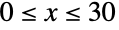 中求解数值方程:
f[x_] = Exp[-100 (x - 10) ^ 2]Sqrt[200 / (2Pi)];
Plot[f[x], {x, 0, 30}, PlotRange -> All]//Quietsol = p /. First[NDSolve[{forward, p[0, t] == p[30, t] == 0, p[x, 0] == f[x]}, p, {x, 0, 30}, {t, 0, 1}, Method -> {"MethodOfLines", "SpatialDiscretization" -> {"TensorProductGrid", "DifferenceOrder" -> "Pseudospectral"}}]]绘制  时柯尔莫哥洛夫前向方程的解,并将其与封闭形式的密度函数进行比较:
Plot[{sol[x, 1], PDF[cir[1], x]}, {x, 0, 30}, PlotRange -> All]使用 Animate 可视化解的动态:
Animate[Plot[sol[x, t], {x, 0, 30}, PlotRange -> {0, 0.3}], {t, 0, 1}, AnimationRunning -> False, TrackedSymbols :> t, SaveDefinitions -> True]用 ItoProcess 表示 GeometricBrownianMotionProcess,其中  表示无风险利率,
 是波动率:
是波动率:
proc = ItoProcess[GeometricBrownianMotionProcess[r, σ, x0]] /. { -> x, -> t}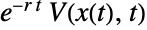
{drift, diffusion} = proc["Derivative", Exp[-r t]V[x[t], t]]经典的 Black–Scholes 方程可以通过使漂移为 0 得到一些化简:
(First[drift]Exp[r t] /. {x[t] -> x}//Simplify) == 0bs = proc["FeynmanKacFormula", r] /. { -> V}用 DSolve 以符号求解 Black–Scholes 方程:
DSolve[{bs, V[x, T] == H[x]}, V[x, t], {x, t}]属性和关系 (2)
把 StratonovichProcess 转化为 ItoProcess:
StratonovichProcess[ⅆx[t] == a[t, x[t]]ⅆt + b[t, x[t]]ⅆw[t], x[t], {x, x0}, t, wWienerProcess[]]ItoProcess[%]StratonovichProcess[%]变换的维纳过程与 ItoProcess 相关:
𝒫1 = TransformedProcess[b[t] ^ 2, bWienerProcess[], t];
𝒫2 = ItoProcess[{0, 1, b[t] ^ 2}, b, t];{Mean[𝒫1[t]] == Mean[𝒫2[t]], Variance[𝒫1[t]] == Variance[𝒫2[t]]}可能存在的问题 (2)
ItoProcess 不支持随机初始条件,所以不能被表示:
ItoProcess[OrnsteinUhlenbeckProcess[μ, σ, θ]]ItoProcess[ⅆx[t] == aⅆt + b x[t]ⅆy[t], x[t], {x, x0}, t, yOrnsteinUhlenbeckProcess[μ, σ, θ]]ItoProcess[OrnsteinUhlenbeckProcess[μ, σ, θ, Subscript[x, 0]]]ItoProcess[ⅆx[t] == aⅆt + b x[t]ⅆy[t], x[t], {x, x0}, t, yOrnsteinUhlenbeckProcess[μ, σ, θ, x0]]驱动过程的起始时间要符合 ItoProcess:
ItoProcess[ⅆx[t] == -x[t] ⅆt + ⅆw[t], x[t], {x, 1}, {t, 3}, wOrnsteinUhlenbeckProcess[0, 1, 1, 1]]//ProcessParameterQItoProcess[ⅆx[t] == -x[t] ⅆt + ⅆw[t], x[t], {x, 1}, {t, 0}, wOrnsteinUhlenbeckProcess[0, 1, 1, 1]]//ProcessParameterQ文本
Wolfram Research (2012),ItoProcess,Wolfram 语言函数,https://reference.wolfram.com/language/ref/ItoProcess.html (更新于 2016 年).
CMS
Wolfram 语言. 2012. "ItoProcess." Wolfram 语言与系统参考资料中心. Wolfram Research. 最新版本 2016. https://reference.wolfram.com/language/ref/ItoProcess.html.
APA
Wolfram 语言. (2012). ItoProcess. Wolfram 语言与系统参考资料中心. 追溯自 https://reference.wolfram.com/language/ref/ItoProcess.html 年