


ListContourPlot3D
ListContourPlot3D[farr]
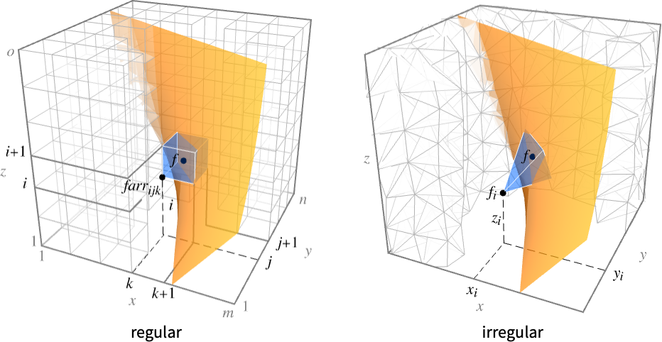
generates a contour plot from an array farr with values farr[[i,j,k]] at points {k,j,i}.
ListContourPlot3D[{{x1,y1,z1,f1},{x2,y2,z2,f2},…}]
generates a contour plot from values fi at point {xi,yi,zi}.
Details and Options
- ListContourPlot3D is also known as an isosurface or level set plot.
- ListContourPlot3D constructs contour surfaces where the interpolated function
 has constant values d1, d2, etc.
 - For regular data, the function
 has value farr[[i,j,k]] at
  .
. - For irregular data,
 has value fi at
  .
. - It visualizes the surfaces
 where the region
  is the Cartesian product
  for regular data and the convex hull of {{x1,y1,z1},…,{xn,yn,zn}} for irregular data.
 - ListContourPlot3D[Tabular[…]cspec] extracts and plots values from the tabular object using the column specification cspec.
- The following forms of column specifications cspec are allowed for plotting tabular data:
-
{colx,coly,colz,colf} plot column f against columns x, y and z - The contour surfaces plotted by ListContourPlot3D can contain disconnected parts.
- By default, ListContourPlot3D shows each contour level as an opaque white surface, with normals pointing outward.
- ListContourPlot3D by default shows three contour levels, equally spaced in f value.
- With the option setting Contours->{f0}, ListContourPlot3D shows only the one contour level f=f0.
- ListContourPlot3D has the same options as Graphics3D, with the following additions and changes: [List of all options]
-
Axes True whether to draw axes BoundaryStyle Automatic how to draw boundaries of regions BoxRatios {1,1,1} bounding 3D box ratios ColorFunction Automatic how to color contour surfaces ColorFunctionScaling True whether to scale arguments to ColorFunction Contours 3 how many or what contour surfaces to show ContourStyle White the style for contour surfaces DataRange Automatic the range of coordinate values to assume for data MaxPlotPoints Automatic the maximum number of points to include Mesh Automatic how many mesh lines in each direction to draw MeshFunctions {#1&,#2&,#3&} how to determine the placement of mesh divisions MeshShading None how to shade regions between mesh lines MeshStyle Automatic the style for mesh divisions Method Automatic the method to use for interpolation and data reduction PerformanceGoal $PerformanceGoal aspects of performance to try to optimize PlotLegends None legends for surfaces PlotRange {Full,Full,Full,Automatic} the range of values to include PlotTheme $PlotTheme overall theme for the plot RegionFunction (True&) how to determine whether a point should be included ScalingFunctions None how to scale individual coordinates TextureCoordinateFunction Automatic how to determine texture coordinates TextureCoordinateScaling True whether to scale arguments to TextureCoordinateFunction - ListContourPlot3D linearly interpolates values to give smooth contours.
- array should be a rectangular array of real numbers; holes will be left in the plot whenever there are elements that are not real numbers.
- ListContourPlot3D[array] by default takes the x, y, and z coordinate values for each data point to be successive integers starting at 1.
- The setting DataRange->{{xmin,xmax},{ymin,ymax},{zmin,zmax}} specifies other ranges of coordinate values to use.
- array can be a SparseArray object.
- The arguments supplied to functions in MeshFunctions and RegionFunction are x, y, z, f. Functions in ColorFunction and TextureCoordinateFunction are by default supplied with scaled versions of these arguments.
- Possible settings for ScalingFunctions include:
-
{sx,sy,sz} scale x, y and z axes - Common built-in scaling functions s include:
-
"Log" 
log scale with automatic tick labeling "Log10" 
base-10 log scale with powers of 10 for ticks "SignedLog" 
log-like scale that includes 0 and negative numbers "Reverse" 
reverse the coordinate direction - ListContourPlot3D returns Graphics3D[GraphicsComplex[data]].
- Themes that affect 3D surfaces include:
-
"DarkMesh" dark mesh lines 
"GrayMesh" gray mesh lines 
"LightMesh" light mesh lines 
"ZMesh" vertically distributed mesh lines 
"ThickSurface" add thickness to surfaces
List of all options
Examples
open all close allBasic Examples (5)
Find a contour in an array of values:
ListContourPlot3D[Table[x ^ 2 + y ^ 2 - z ^ 2 + RandomReal[0.1], {x, -2, 2, 0.2}, {y, -2, 2, 0.2}, {z, -2, 2, 0.2}], Contours -> {0}, Mesh -> None]ListContourPlot3D[Table[x ^ 2 + y ^ 2 - z ^ 2 + RandomReal[0.1], {x, -2, 2, 0.2}, {y, -2, 2, 0.2}, {z, -2, 2, 0.2}], Contours -> 3, Mesh -> None]Find a contour from irregular data:
data = Table[{x = RandomReal[{-1, 1}], y = RandomReal[{-1, 1}], z = RandomReal[{-1, 1}], x ^ 2 + y ^ 2 - z ^ 2}, {5000}];ListContourPlot3D[data, Contours -> {0.5}, Mesh -> None]ListContourPlot3D[Table[x ^ 2 + y ^ 2 - z ^ 2 + RandomReal[0.1], {x, -2, 2, 0.2}, {y, -2, 2, 0.2}, {z, -2, 2, 0.2}], Contours -> 3, Mesh -> None, ContourStyle -> {Red, Orange, Yellow}]Use legends to identify contours by color:
ListContourPlot3D[Table[x ^ 2 + y ^ 2 - z ^ 2, {x, -2, 2, 0.2}, {y, -2, 2, 0.2}, {z, -2, 2, 0.2}], Contours -> 5, Mesh -> None, PlotLegends -> "Expressions"]Scope (7)
Data (5)
For regular data consisting of ![]() values, the
values, the ![]() ,
, ![]() , and
, and ![]() data ranges are taken to be integer values:
data ranges are taken to be integer values:
ListContourPlot3D[Table[Sqrt[x ^ 2 + y ^ 2 + z ^ 2], {x, 0, 3, 0.1}, {y, 0, 3, 0.1}, {z, 0, 3, 0.1}]]Provide explicit ![]() ,
, ![]() , and
, and ![]() data ranges by using DataRange:
data ranges by using DataRange:
ListContourPlot3D[Table[Sqrt[x ^ 2 + y ^ 2 + z ^ 2], {x, 0, 3, 0.1}, {y, 0, 3, 0.1}, {z, 0, 3, 0.1}], DataRange -> {{0, 3}, {0, 3}, {0, 3}}]For irregular data consisting of ![]() triples, the
triples, the ![]() ,
, ![]() , and
, and ![]() data ranges are inferred from data:
data ranges are inferred from data:
data = Table[{x = RandomReal[{-1, 1}], y = RandomReal[{0, 1}], z = RandomReal[{-1, 1}], Sqrt[x ^ 2 + y ^ 2 + z ^ 2]}, {1000}];ListContourPlot3D[data, Mesh -> All]Use MaxPlotPoints to limit the number of points used:
Table[ListContourPlot3D[Table[Sqrt[x ^ 2 + y ^ 2 + z ^ 2], {x, 0, 3, 0.1}, {y, 0, 3, 0.1}, {z, 0, 3, 0.1}], MaxPlotPoints -> mp, Mesh -> All], {mp, {Infinity, 15, 5}}]Use data with a different unit for each dimension:
data = Table[{Quantity[x = RandomReal[{-1, 1}], "Meters"], Quantity[y = RandomReal[{-1, 1}], "Seconds"], Quantity[z = RandomReal[{-1, 1}], "Kilograms"], x ^ 2 + y ^ 2 - z ^ 2}, {1000}];ListContourPlot3D[data, BoxRatios -> Automatic, Contours -> {0}, AxesLabel -> Automatic]ListContourPlot3D[data, AxesLabel -> Automatic, Contours -> {0}, TargetUnits -> {"Feet", "Seconds", "Pounds", Automatic}]Tabular Data (1)
tabular = Tabular[IconizedObject[«data»], {"f", "x", "y", "z"}]Plot tabular data in which each column represents data in the form {x,y,z,f}:
ListContourPlot3D[tabular -> {"x", "y", "z", "f"}]Include a legend for the plot:
ListContourPlot3D[tabular -> {"x", "y", "z", "f"}, PlotLegends -> Automatic]Options (93)
Axes (3)
By default, Axes are drawn for ListContourPlot3D:
ListContourPlot3D[Table[Sqrt[x ^ 2 + y ^ 2 + z ^ 2], {x, 0, 3, 0.1}, {y, 0, 3, 0.1}, {z, 0, 3, 0.1}]]Use AxesFalse to turn off axes:
ListContourPlot3D[Table[Sqrt[x ^ 2 + y ^ 2 + z ^ 2], {x, 0, 3, 0.1}, {y, 0, 3, 0.1}, {z, 0, 3, 0.1}], Axes -> False]Turn each axis on individually:
{ListContourPlot3D[Table[Sqrt[x ^ 2 + y ^ 2 + z ^ 2], {x, 0, 3, 0.1}, {y, 0, 3, 0.1}, {z, 0, 3, 0.1}], Axes -> {True, False, False}], ListContourPlot3D[Table[Sqrt[x ^ 2 + y ^ 2 + z ^ 2], {x, 0, 3, 0.1}, {y, 0, 3, 0.1}, {z, 0, 3, 0.1}], Axes -> {False, True, False}], ListContourPlot3D[Table[Sqrt[x ^ 2 + y ^ 2 + z ^ 2], {x, 0, 3, 0.1}, {y, 0, 3, 0.1}, {z, 0, 3, 0.1}], Axes -> {False, False, True}]}AxesLabel (4)
No axes labels are drawn by default:
ListContourPlot3D[Table[x ^ 2 + y ^ 2 + z ^ 2, {z, -1, 1, 0.02}, {y, -1, 1, 0.02}, {x, -1, 1, 0.02}]]ListContourPlot3D[Table[x ^ 2 + y ^ 2 + z ^ 2, {z, -1, 1, 0.02}, {y, -1, 1, 0.02}, {x, -1, 1, 0.02}], AxesLabel -> z]ListContourPlot3D[Table[x ^ 2 + y ^ 2 + z ^ 2, {z, -1, 1, 0.02}, {y, -1, 1, 0.02}, {x, -1, 1, 0.02}], AxesLabel -> {"x", "y", "z"}]data = Table[{Quantity[x = RandomReal[{-1, 1}], "Meters"], Quantity[y = RandomReal[{-1, 1}], "Seconds"], Quantity[z = RandomReal[{-1, 1}], "Kilograms"], x ^ 2 + y ^ 2 - z ^ 2}, {1000}];ListContourPlot3D[data, BoxRatios -> Automatic, Contours -> {0}, AxesLabel -> Automatic]AxesOrigin (2)
The position of the axes is determined automatically:
ListContourPlot3D[Table[x ^ 2 + y ^ 2 + z ^ 2, {z, -1, 1, 0.02}, {y, -1, 1, 0.02}, {x, -1, 1, 0.02}]]Specify an explicit origin for the axes:
ListContourPlot3D[Table[x ^ 2 + y ^ 2 + z ^ 2, {z, -1, 1, 0.02}, {y, -1, 1, 0.02}, {x, -1, 1, 0.02}], AxesOrigin -> {100, 0, 100}]AxesStyle (4)
Change the style for the axes:
ListContourPlot3D[Table[Sqrt[x ^ 2 + y ^ 2 + z ^ 2], {x, 0, 3, 0.1}, {y, 0, 3, 0.1}, {z, 0, 3, 0.1}], AxesStyle -> Red]Specify the style of each axis:
ListContourPlot3D[Table[Sqrt[x ^ 2 + y ^ 2 + z ^ 2], {x, 0, 3, 0.1}, {y, 0, 3, 0.1}, {z, 0, 3, 0.1}], AxesStyle -> {{Thick, Brown}, {Thick, Blue}, {Thick, Green}}]Use different styles for the ticks and the axes:
ListContourPlot3D[Table[Sqrt[x ^ 2 + y ^ 2 + z ^ 2], {x, 0, 3, 0.1}, {y, 0, 3, 0.1}, {z, 0, 3, 0.1}], AxesStyle -> Green, TicksStyle -> Red]Use different styles for the labels and the axes:
ListContourPlot3D[Table[Sqrt[x ^ 2 + y ^ 2 + z ^ 2], {x, 0, 3, 0.1}, {y, 0, 3, 0.1}, {z, 0, 3, 0.1}], AxesStyle -> Green, LabelStyle -> Red]BoundaryStyle (3)
Use a red boundary around the edges of the contours:
ListContourPlot3D[Table[Sqrt[x ^ 2 + y ^ 2 + z ^ 2], {x, 0, 3, 0.1}, {y, 0, 3, 0.1}, {z, 0, 3, 0.1}], BoundaryStyle -> Red, Mesh -> None]Use None to omit the boundary:
ListContourPlot3D[Table[Sqrt[x ^ 2 + y ^ 2 + z ^ 2], {x, 0, 3, 0.1}, {y, 0, 3, 0.1}, {z, 0, 3, 0.1}], BoundaryStyle -> None, Mesh -> None]BoundaryStyle applies to holes cut by RegionFunction:
ListContourPlot3D[Table[Sqrt[x ^ 2 + y ^ 2 + z ^ 2], {x, -3, 3, 0.1}, {y, -3, 3, 0.1}, {z, -3, 3, 0.1}], DataRange -> {{-3, 3}, {-3, 3}, {-3, 3}}, BoundaryStyle -> Red, Mesh -> None, RegionFunction -> Function[{x, y, z, w}, x < 0 || y > 0]]BoxRatios (3)
By default, the edges of the bounding box have the same length:
ListContourPlot3D[Table[{x = RandomReal[{-1, 1}], y = RandomReal[{-2, 2}], z = RandomReal[{-0.5, 0.5}], x ^ 2 + (y / 2) ^ 2 + (2z) ^ 2}, {2500}]]Specify the ratios between the bounding box lengths:
ListContourPlot3D[Table[{x = RandomReal[{-1, 1}], y = RandomReal[{-2, 2}], z = RandomReal[{-0.5, 0.5}], x ^ 2 + (y / 2) ^ 2 + (2z) ^ 2}, {2500}], BoxRatios -> {1, 2, 1 / 2}]Use the actual coordinate values for the ratios:
ListContourPlot3D[Table[{x = RandomReal[{-1, 1}], y = RandomReal[{-2, 2}], z = RandomReal[{-0.5, 0.5}], x ^ 2 + (y / 2) ^ 2 + (2z) ^ 2}, {2500}], BoxRatios -> Automatic]ColorFunction (5)
Color the contours according to the ![]() ,
, ![]() ,
, ![]() , or
, or ![]() values:
values:
Table[ListContourPlot3D[Table[x ^ 2 + y ^ 2 + z ^ 2, {x, -3, 3, 0.1}, {y, -3, 3, 0.1}, {z, -3, 3, 0.1}], ColorFunction -> Function[{x, y, z, f}, Evaluate[c]], PlotLabel -> c, Axes -> None], {c, {Hue[x], Hue[y], Hue[z], Hue[f]}}]ListContourPlot3D[Table[x ^ 2 + y ^ 2 + z ^ 2, {x, -3, 3, 0.1}, {y, -3, 3, 0.1}, {z, -3, 3, 0.1}], Mesh -> None, Contours -> 4, ColorFunction -> "DarkRainbow"]ColorFunction has higher priority than ContourStyle:
ListContourPlot3D[Table[x ^ 2 + y ^ 2 + z ^ 2, {x, -3, 3, 0.1}, {y, -3, 3, 0.1}, {z, -3, 3, 0.1}], Mesh -> None, Contours -> 4, ColorFunction -> "DarkRainbow", ContourStyle -> Directive[Opacity[0.5], Red]]ListContourPlot3D[Table[x ^ 2 + y ^ 2 + z ^ 2, {x, -3, 3, 0.1}, {y, -3, 3, 0.1}, {z, -3, 3, 0.1}], DataRange -> {{-3, 3}, {-3, 3}, {-3, 3}}, ColorFunction -> Function[{x, y, z, f}, If[z < 0, Red, Green]], ColorFunctionScaling -> False]ColorFunction has lower priority than MeshShading:
ListContourPlot3D[Table[x ^ 2 + y ^ 2 + z ^ 2, {x, -3, 3, 0.1}, {y, -3, 3, 0.1}, {z, -3, 3, 0.1}], ColorFunction -> Function[{x, y, z, f}, Hue[z]], MeshFunctions -> {#3&}, MeshShading -> {Automatic, StandardGray}]ColorFunctionScaling (2)
Use unscaled values to color the contours:
ListContourPlot3D[Table[x ^ 2 + y ^ 2 + z ^ 2, {x, -3, 3, 0.1}, {y, -3, 3, 0.1}, {z, -3, 3, 0.1}], Mesh -> None, Contours -> 4, ColorFunction -> Function[{x, y, z, f}, Hue[f / 5]], ColorFunctionScaling -> False]Use an overlay density based on the coordinate values:
ListContourPlot3D[Table[x ^ 2 + y ^ 2 + z ^ 2, {x, -3, 3, 0.1}, {y, -3, 3, 0.1}, {z, -3, 3, 0.1}], DataRange -> {{-3, 3}, {-3, 3}, {-3, 3}}, ColorFunction -> Function[{x, y, z, f}, Hue[Sin[x]Sin[y]]], ColorFunctionScaling -> False, Mesh -> None]Contours (3)
Use five equally spaced contours:
ListContourPlot3D[Table[x ^ 3 + y ^ 2 - z ^ 2, {z, -2, 2, 0.1}, {y, -2, 2, 0.1}, {x, -2, 2, 0.1}], Contours -> 5, Mesh -> None]Use automatic contour selection:
ListContourPlot3D[Table[x ^ 3 + y ^ 2 - z ^ 2, {z, -2, 2, 0.1}, {y, -2, 2, 0.1}, {x, -2, 2, 0.1}], Contours -> Automatic, Mesh -> None]ListContourPlot3D[Table[x ^ 3 + y ^ 2 - z ^ 2, {z, -2, 2, 0.1}, {y, -2, 2, 0.1}, {x, -2, 2, 0.1}], Contours -> {-2, 2}, Mesh -> None]ContourStyle (7)
ListContourPlot3D[Table[x ^ 2 + y ^ 2 + z ^ 2, {z, -2, 2, 0.1}, {y, -2, 2, 0.1}, {x, -2, 2, 0.1}], Mesh -> None, ContourStyle -> Opacity[0.5]]Use distinct colors for each contour:
ListContourPlot3D[Table[x ^ 2 + y ^ 2 + z ^ 2, {z, -2, 2, 0.1}, {y, -2, 2, 0.1}, {x, -2, 2, 0.1}], Mesh -> None, ContourStyle -> {Red, Green, Blue}]Use FaceForm to get different colors on the inside and outside:
ListContourPlot3D[Table[x ^ 2 + y ^ 2 - z ^ 2, {z, -2, 2, 0.1}, {y, -2, 2, 0.1}, {x, -2, 2, 0.1}], Contours -> {1}, Mesh -> 5, ContourStyle -> {FaceForm[Yellow, Blue]}]Alternate styles for contour surfaces:
ListContourPlot3D[Table[x ^ 2 + y ^ 2 + z ^ 2, {z, -2, 2, 0.1}, {y, -2, 2, 0.1}, {x, -2, 2, 0.1}], Contours -> 4, Mesh -> None, ContourStyle -> {Blue, Opacity[0.5]}]Use the same style for all the contours:
ListContourPlot3D[Table[x ^ 2 + y ^ 2 + z ^ 2, {z, -2, 2, 0.1}, {y, -2, 2, 0.1}, {x, -2, 2, 0.1}], Contours -> 6, Mesh -> None, ContourStyle -> Directive[Opacity[0.5], Orange]]ColorFunction has higher priority than ContourStyle:
ListContourPlot3D[Table[x ^ 2 + y ^ 2 - z ^ 2, {z, -2, 2, 0.1}, {y, -2, 2, 0.1}, {x, -2, 2, 0.1}], Contours -> {1}, Mesh -> None, ContourStyle -> Directive[Opacity[0.5], Red], ColorFunction -> Function[{x, y, z, f}, Hue[z]]]MeshShading has higher priority than ContourStyle:
ListContourPlot3D[Table[x ^ 2 + y ^ 2 - z ^ 2, {z, -2, 2, 0.1}, {y, -2, 2, 0.1}, {x, -2, 2, 0.1}], Contours -> {1}, MeshFunctions -> {#3&}, ContourStyle -> Directive[Opacity[0.5], Yellow], MeshShading -> {Red, Automatic}]DataRange (3)
Arrays of values are displayed against the number of elements in each direction:
ListContourPlot3D[Table[x ^ 3 + y ^ 2 - z ^ 2, {z, -2, 2, 0.1}, {y, -2, 2, 0.1}, {x, -2, 2, 0.1}]]Rescale to the sampling space:
ListContourPlot3D[Table[x ^ 3 + y ^ 2 - z ^ 2, {z, -2, 2, 0.1}, {y, -2, 2, 0.1}, {x, -2, 2, 0.1}], DataRange -> {{-2, 2}, {-2, 2}, {-2, 2}}]Tuples are interpreted as ![]() ,
, ![]() ,
, ![]() ,
, ![]() coordinates:
coordinates:
data = Table[{x = RandomReal[{-2, 2}], y = RandomReal[{-2, 2}], z = RandomReal[{-2, 2}], x ^ 3 + y ^ 2 - z ^ 2}, {2500}];ListContourPlot3D[data]ImageSize (7)
Use named sizes such as Tiny, Small, Medium and Large:
{ListContourPlot3D[Table[Sqrt[x ^ 2 + y ^ 2 + z ^ 2], {x, 0, 3, 0.1}, {y, 0, 3, 0.1}, {z, 0, 3, 0.1}], ImageSize -> Tiny], ListContourPlot3D[Table[Sqrt[x ^ 2 + y ^ 2 + z ^ 2], {x, 0, 3, 0.1}, {y, 0, 3, 0.1}, {z, 0, 3, 0.1}], ImageSize -> Small]}Specify the width of the plot:
{ListContourPlot3D[Table[Sqrt[x ^ 2 + y ^ 2 + z ^ 2], {x, 0, 3, 0.1}, {y, 0, 3, 0.1}, {z, 0, 3, 0.1}], ImageSize -> 150], ListContourPlot3D[Table[Sqrt[x ^ 2 + y ^ 2 + z ^ 2], {x, 0, 3, 0.1}, {y, 0, 3, 0.1}, {z, 0, 3, 0.1}], AspectRatio -> 1.5, ImageSize -> 150]}Specify the height of the plot:
{ListContourPlot3D[Table[Sqrt[x ^ 2 + y ^ 2 + z ^ 2], {x, 0, 3, 0.1}, {y, 0, 3, 0.1}, {z, 0, 3, 0.1}], ImageSize -> {Automatic, 150}], ListContourPlot3D[Table[Sqrt[x ^ 2 + y ^ 2 + z ^ 2], {x, 0, 3, 0.1}, {y, 0, 3, 0.1}, {z, 0, 3, 0.1}], AspectRatio -> 2, ImageSize -> {Automatic, 150}]}Allow the width and height to be up to a certain size:
{ListContourPlot3D[Table[Sqrt[x ^ 2 + y ^ 2 + z ^ 2], {x, 0, 3, 0.1}, {y, 0, 3, 0.1}, {z, 0, 3, 0.1}], ImageSize -> UpTo[200]], ListContourPlot3D[Table[Sqrt[x ^ 2 + y ^ 2 + z ^ 2], {x, 0, 3, 0.1}, {y, 0, 3, 0.1}, {z, 0, 3, 0.1}], AspectRatio -> 2, ImageSize -> UpTo[200]]}Specify the width and height for a graphic, padding with space if necessary:
ListContourPlot3D[Table[Sqrt[x ^ 2 + y ^ 2 + z ^ 2], {x, 0, 3, 0.1}, {y, 0, 3, 0.1}, {z, 0, 3, 0.1}], ImageSize -> {200, 250}, Background -> StandardGray]Setting AspectRatioFull will fill the available space:
ListContourPlot3D[Table[Sqrt[x ^ 2 + y ^ 2 + z ^ 2], {x, 0, 3, 0.1}, {y, 0, 3, 0.1}, {z, 0, 3, 0.1}], AspectRatio -> Full, ImageSize -> {200, 250}, Background -> StandardGray]Use maximum sizes for the width and height:
{ListContourPlot3D[Table[Sqrt[x ^ 2 + y ^ 2 + z ^ 2], {x, 0, 3, 0.1}, {y, 0, 3, 0.1}, {z, 0, 3, 0.1}], ImageSize -> {UpTo[150], UpTo[150]}], ListContourPlot3D[Table[Sqrt[x ^ 2 + y ^ 2 + z ^ 2], {x, 0, 3, 0.1}, {y, 0, 3, 0.1}, {z, 0, 3, 0.1}], AspectRatio -> 2, ImageSize -> {UpTo[150], UpTo[150]}]}Use ImageSizeFull to fill the available space in an object:
Framed[Pane[ListContourPlot3D[Table[Sqrt[x ^ 2 + y ^ 2 + z ^ 2], {x, 0, 3, 0.1}, {y, 0, 3, 0.1}, {z, 0, 3, 0.1}], ImageSize -> Full, Background -> StandardGray], {200, 100}]]Specify the image size as a fraction of the available space:
Framed[Pane[ListContourPlot3D[Table[Sqrt[x ^ 2 + y ^ 2 + z ^ 2], {x, 0, 3, 0.1}, {y, 0, 3, 0.1}, {z, 0, 3, 0.1}], AspectRatio -> Full, ImageSize -> {Scaled[0.5], Scaled[0.5]}, Background -> StandardGray], {200, 200}]]MaxPlotPoints (3)
ListContourPlot normally uses all of the points in the dataset:
ListContourPlot3D[Table[x ^ 3 + y ^ 2 - z ^ 2, {z, -2, 2, 0.1}, {y, -2, 2, 0.1}, {x, -2, 2, 0.1}], Mesh -> All]data = Table[{x = RandomReal[{-2, 2}], y = RandomReal[{-2, 2}], z = RandomReal[{-2, 2}], x ^ 3 + y ^ 2 - z ^ 2}, {5000}];ListContourPlot3D[data, Mesh -> All]Limit the number of points used in each direction:
ListContourPlot3D[Table[x ^ 3 + y ^ 2 - z ^ 2, {z, -2, 2, 0.1}, {y, -2, 2, 0.1}, {x, -2, 2, 0.1}], MaxPlotPoints -> 10, Mesh -> All]MaxPlotPoints imposes a regular grid on irregular data:
data = Table[{x = RandomReal[{-2, 2}], y = RandomReal[{-2, 2}], z = RandomReal[{-2, 2}], x ^ 3 + y ^ 2 - z ^ 2}, {5000}];ListContourPlot3D[data, MaxPlotPoints -> 10, Mesh -> All]Mesh (6)
ListContourPlot3D[Table[x ^ 3 + y ^ 2 - z ^ 2, {z, -2, 2, 0.1}, {y, -2, 2, 0.1}, {x, -2, 2, 0.1}], Mesh -> All]Use None to not draw any mesh:
ListContourPlot3D[Table[x ^ 3 + y ^ 2 - z ^ 2, {z, -2, 2, 0.1}, {y, -2, 2, 0.1}, {x, -2, 2, 0.1}], Mesh -> None]Use five mesh levels in each direction:
ListContourPlot3D[Table[x ^ 3 + y ^ 2 - z ^ 2, {z, -2, 2, 0.1}, {y, -2, 2, 0.1}, {x, -2, 2, 0.1}], Mesh -> 5, MeshFunctions -> {#1&, #2&, #3&}]Use five mesh levels in the ![]() direction and 10 in the
direction and 10 in the ![]() direction:
direction:
ListContourPlot3D[Table[x ^ 3 + y ^ 2 - z ^ 2, {z, -2, 2, 0.1}, {y, -2, 2, 0.1}, {x, -2, 2, 0.1}], Mesh -> {5, 10}, MeshFunctions -> {#1&, #2&}]Use mesh lines at specific values:
ListContourPlot3D[Table[x ^ 2 + y ^ 2 + z ^ 2, {z, -2, 2, 0.1}, {y, -2, 2, 0.1}, {x, -2, 2, 0.1}], DataRange -> {{-2, 2}, {-2, 2}, {-2, 2}}, Contours -> {1}, Mesh -> {{0}, {0}}, MeshFunctions -> {#1&, #2&}]Use different styles for different mesh lines:
ListContourPlot3D[Table[x ^ 2 + y ^ 2 + z ^ 2, {z, -2, 2, 0.1}, {y, -2, 2, 0.1}, {x, -2, 2, 0.1}], DataRange -> {{-2, 2}, {-2, 2}, {-2, 2}}, Contours -> {1}, Mesh -> {{{0, Thick}}, {{0, Red}}}]MeshFunctions (2)
Use a mesh evenly spaced in the ![]() ,
, ![]() , and
, and ![]() directions:
directions:
Table[ListContourPlot3D[Table[x ^ 2 + y ^ 2 + z ^ 2, {z, -2, 2, 0.1}, {y, -2, 2, 0.1}, {x, -2, 2, 0.1}], DataRange -> {{-2, 2}, {-2, 2}, {-2, 2}}, Contours -> {1}, PlotLabel -> f, MeshFunctions -> {Function[{x, y, z}, f]}, Axes -> None], {f, {x, y, z}}]Mesh with respect to radial distance:
ListContourPlot3D[Table[x ^ 3 + y ^ 2 - z ^ 2, {z, -2, 2, 0.1}, {y, -2, 2, 0.1}, {x, -2, 2, 0.1}], DataRange -> {{-2, 2}, {-2, 2}, {-2, 2}}, MeshFunctions -> (Norm[{#1, #2, #3}]&)]MeshShading (5)
Alternate red and blue sections in the ![]() direction:
direction:
ListContourPlot3D[Table[x ^ 2 + y ^ 2 - z ^ 2, {z, -2, 2, 0.1}, {y, -2, 2, 0.1}, {x, -2, 2, 0.1}], Contours -> {1}, MeshFunctions -> {#3&}, MeshShading -> {Red, Blue}]MeshShading has higher priority than ContourStyle for styling:
ListContourPlot3D[Table[x ^ 2 + y ^ 2 - z ^ 2, {z, -2, 2, 0.1}, {y, -2, 2, 0.1}, {x, -2, 2, 0.1}], Contours -> 1, MeshFunctions -> {#3&}, MeshShading -> {None, Blue}]Use ContourStyle for some segments by setting MeshShading to Automatic:
ListContourPlot3D[Table[x ^ 2 + y ^ 2 - z ^ 2, {z, -2, 2, 0.1}, {y, -2, 2, 0.1}, {x, -2, 2, 0.1}], Contours -> {1}, MeshFunctions -> {#3&}, MeshShading -> {Red, Automatic}, ContourStyle -> Directive[Opacity[0.5], Yellow]]MeshShading can be used with ColorFunction:
ListContourPlot3D[Table[x ^ 2 + y ^ 2 - z ^ 2, {z, -2, 2, 0.1}, {y, -2, 2, 0.1}, {x, -2, 2, 0.1}], Contours -> {1}, MeshFunctions -> {#3&}, MeshShading -> {StandardGray, Automatic}, ColorFunction -> Function[{x, y, z, f}, Hue[z]]]Fill between regions defined by multiple mesh functions:
ListContourPlot3D[Table[x ^ 2 + y ^ 2 - z ^ 2, {z, -2, 2, 0.1}, {y, -2, 2, 0.1}, {x, -2, 2, 0.1}], Contours -> {1}, Mesh -> 5, Lighting -> "Neutral", MeshShading -> Table[RGBColor[r, g, b], {r, 0, 1, 1 / 5}, {g, 0, 1, 1 / 5}, {b, 0, 1, 1 / 5}]]MeshStyle (2)
Use a dashed mesh in the ![]() direction:
direction:
ListContourPlot3D[Table[x ^ 2 + y ^ 2 - z ^ 2, {z, -2, 2, 0.1}, {y, -2, 2, 0.1}, {x, -2, 2, 0.1}], Contours -> {1}, MeshFunctions -> {#1&}, MeshStyle -> Dashed, Mesh -> 5]Use a dashed mesh in the ![]() direction and a blue mesh in the
direction and a blue mesh in the ![]() direction:
direction:
ListContourPlot3D[Table[x ^ 2 + y ^ 2 - z ^ 2, {z, -2, 2, 0.1}, {y, -2, 2, 0.1}, {x, -2, 2, 0.1}], Contours -> {1}, Mesh -> 5, MeshFunctions -> {#1&, #2&}, MeshStyle -> {Dashed, Blue}]PerformanceGoal (2)
Generate a higher-quality plot:
Timing[ListContourPlot3D[Table[x ^ 2 + y ^ 2 - z ^ 2, {z, -2, 2, 0.1}, {y, -2, 2, 0.1}, {x, -2, 2, 0.1}], PerformanceGoal -> "Quality"]]Emphasize performance, possibly at the cost of quality:
Timing[ListContourPlot3D[Table[x ^ 2 + y ^ 2 - z ^ 2, {z, -2, 2, 0.1}, {y, -2, 2, 0.1}, {x, -2, 2, 0.1}], PerformanceGoal -> "Speed"]]PlotRange (2)
Show the contours over the full ![]() ,
, ![]() ,
, ![]() range:
range:
ListContourPlot3D[Table[x ^ 2 + y ^ 2 + z ^ 2, {z, -2, 2, 0.1}, {y, -2, 2, 0.1}, {x, -2, 2, 0.1}], DataRange -> {{-2, 2}, {-2, 2}, {-2, 2}}, Contours -> 5]Use specific ranges to show more detail:
ListContourPlot3D[Table[x ^ 2 + y ^ 2 + z ^ 2, {z, -2, 2, 0.1}, {y, -2, 2, 0.1}, {x, -2, 2, 0.1}], DataRange -> {{-2, 2}, {-2, 2}, {-2, 2}}, Contours -> 5, PlotRange -> {{-2, 0}, {-2, 2}, {-2, 2}}, BoxRatios -> Automatic]PlotTheme (3)
ListContourPlot3D[Table[x ^ 2 + y ^ 2 - z ^ 2, {z, -2, 2, 0.1}, {y, -2, 2, 0.1}, {x, -2, 2, 0.1}], PlotTheme -> "Marketing"]Adjust the appearance by removing the ticks and some mesh lines:
ListContourPlot3D[Table[x ^ 2 + y ^ 2 - z ^ 2, {z, -2, 2, 0.1}, {y, -2, 2, 0.1}, {x, -2, 2, 0.1}], PlotTheme -> "Marketing", Ticks -> None, Mesh -> 5]Create a thick surface for 3D printing:
ListContourPlot3D[Table[x ^ 2 + y ^ 2 - z ^ 2, {z, -2, 2, 0.1}, {y, -2, 2, 0.1}, {x, -2, 2, 0.1}], Contours -> {0}, PlotTheme -> "ThickSurface"]RegionFunction (2)
Table[ListContourPlot3D[Table[x ^ 2 + y ^ 2 + z ^ 2, {z, -1, 1, 0.02}, {y, -1, 1, 0.02}, {x, -1, 1, 0.02}], DataRange -> {{-1, 1}, {-1, 1}, {-1, 1}}, Mesh -> None, Axes -> None, Contours -> 4, RegionFunction -> Function[{x, y, z}, Evaluate[f]], PlotLabel -> f], {f, {-1 / 2 < x < 1 / 2, -1 / 2 < y < 1 / 2, -1 / 2 < z < 1 / 2}}]Remove a wedge to see hidden features:
ListContourPlot3D[Table[x ^ 2 + y ^ 2 + z ^ 2, {z, -1, 1, 0.02}, {y, -1, 1, 0.02}, {x, -1, 1, 0.02}], DataRange -> {{-1, 1}, {-1, 1}, {-1, 1}}, Contours -> 4, Mesh -> None, Axes -> None, RegionFunction -> Function[{x, y, z}, x < 0 || y > 0]]ScalingFunctions (4)
By default, ContourPlot3D uses linear scales in all directions:
ListContourPlot3D[Table[x ^ 2 + y ^ 2 - z, {z, 1, 10, 0.1}, {y, -2, 2, 0.1}, {x, -2, 2, 0.1}]]Use a log scale in the ![]() direction:
direction:
ListContourPlot3D[Table[x ^ 2 + y ^ 2 - z, {z, 1, 10, 0.1}, {y, -2, 2, 0.1}, {x, -2, 2, 0.1}], ScalingFunctions -> {None, None, "Log"}, PlotRange -> All]Reverse the coordinate direction of the ![]() axis:
axis:
ListContourPlot3D[Table[x ^ 2 + y ^ 2 - z, {z, 1, 10, 0.1}, {y, -2, 2, 0.1}, {x, -2, 2, 0.1}], ScalingFunctions -> {None, None, "Reverse"}]Use a scale defined by a function, specifying the function and its inverse:
ListContourPlot3D[Table[x ^ 2 + y ^ 2 - z, {z, 1, 10, 0.1}, {y, -2, 2, 0.1}, {x, -2, 2, 0.1}], ScalingFunctions -> {None, None, {-Log[# + 1]&, Exp[-#] - 1&}}]TargetUnits (1)
Units are automatically determined from the data:
data = Table[{Quantity[x = RandomReal[{-1, 1}], "Meters"], Quantity[y = RandomReal[{-1, 1}], "Seconds"], Quantity[z = RandomReal[{-1, 1}], "Kilograms"], x ^ 2 + y ^ 2 - z ^ 2}, {1000}];ListContourPlot3D[data, BoxRatios -> Automatic, Contours -> {0}, AxesLabel -> Automatic]ListContourPlot3D[data, AxesLabel -> Automatic, Contours -> {0}, TargetUnits -> {"Feet", "Seconds", "Pounds", Automatic}]TextureCoordinateFunction (5)
Textures use scaled ![]() and
and ![]() coordinates by default:
coordinates by default:
ListContourPlot3D[Table[x ^ 2 + y ^ 2 - z ^ 2, {x, -2, 2, 0.1}, {y, -2, 2, 0.1}, {z, -2, 2, 0.1}], Contours -> {1}, Mesh -> None, Lighting -> "Neutral", ContourStyle -> Texture[ExampleData[{"ColorTexture", "WavesPattern"}]]]ListContourPlot3D[Table[x ^ 2 + y ^ 2 - z ^ 2, {x, -2, 2, 0.1}, {y, -2, 2, 0.1}, {z, -2, 2, 0.1}], Contours -> {1}, Mesh -> None, Lighting -> "Neutral", TextureCoordinateFunction -> ({#1, #3}&), ContourStyle -> Texture[ExampleData[{"ColorTexture", "WavesPattern"}]]]Use different textures for different surfaces:
ListContourPlot3D[Table[x ^ 2 + y ^ 2 - z ^ 2, {x, -2, 2, 0.1}, {y, -2, 2, 0.1}, {z, -2, 2, 0.1}], Mesh -> None, Lighting -> "Neutral", ContourStyle -> {Texture[ExampleData[{"ColorTexture", "Ash"}]], Texture[ExampleData[{"ColorTexture", "Amboyna"}]], Texture[ExampleData[{"ColorTexture", "Laurel"}]]}]ListContourPlot3D[Table[x ^ 2 + y ^ 2 - z ^ 2, {x, -2, 2, 0.1}, {y, -2, 2, 0.1}, {z, -2, 2, 0.1}], Contours -> {1}, Mesh -> None, Lighting -> "Neutral", TextureCoordinateScaling -> False, ContourStyle -> Texture[ExampleData[{"ColorTexture", "WavesPattern"}]]]Use textures to highlight how parameters map onto a surface:
texture = ArrayPlot[{{1, 1, 1, 2, 1, 1}, {2, 0, 0, 2, 0, 0}, {2, 0, 0, 2, 0, 0}, {2, 1, 1, 1, 1, 1}, {2, 0, 0, 2, 0, 0}, {2, 0, 0, 2, 0, 0}}, ColorRules -> {1 -> Red, 2 -> Blue, 0 -> White}, Frame -> False, PlotRangePadding -> None, ImagePadding -> None, ImageSize -> 100]ListContourPlot3D[Table[x ^ 2 + y ^ 2 - z ^ 2, {x, -2, 2, 0.1}, {y, -2, 2, 0.1}, {z, -2, 2, 0.1}], Contours -> {1}, Mesh -> None, Lighting -> "Neutral", ContourStyle -> Texture[texture]]TextureCoordinateScaling (1)
Use scaled or unscaled coordinates for textures:
texture = ArrayPlot[{{1, 1, 1, 2, 1, 1}, {2, 0, 0, 2, 0, 0}, {2, 0, 0, 2, 0, 0}, {2, 1, 1, 1, 1, 1}, {2, 0, 0, 2, 0, 0}, {2, 0, 0, 2, 0, 0}}, ColorRules -> {1 -> Red, 2 -> Blue, 0 -> White}, Frame -> False, PlotRangePadding -> None, ImagePadding -> None, ImageSize -> 100]Table[ListContourPlot3D[Table[x ^ 2 + y ^ 2 - z ^ 2, {x, -2, 2, 0.1}, {y, -2, 2, 0.1}, {z, -2, 2, 0.1}], Mesh -> None, Lighting -> "Neutral", ContourStyle -> Texture[texture], TextureCoordinateScaling -> s, PlotLabel -> s], {s, {True, False}}]Ticks (6)
Ticks are placed automatically in each plot:
ListContourPlot3D[Table[x ^ 2 + y ^ 2 - z ^ 2, {x, -2, 2, 0.2}, {y, -2, 2, 0.2}, {z, -4, 4, .2}], Mesh -> None]Use TicksNone to not draw any tick marks:
ListContourPlot3D[Table[x ^ 2 + y ^ 2 - z ^ 2, {x, -2, 2, 0.2}, {y, -2, 2, 0.2}, {z, -4, 4, .2}], Mesh -> None, Ticks -> None]Place tick marks at specific positions:
ListContourPlot3D[Table[x ^ 2 + y ^ 2 - z ^ 2, {x, -2, 2, 0.2}, {y, -2, 2, 0.2}, {z, -4, 4, .2}], Mesh -> None, Ticks -> {{0, 20, 40}, {0, 10, 20}, {0, 10, 20}}]Draw tick marks at the specified positions with the specified labels:
ListContourPlot3D[Table[x ^ 2 + y ^ 2 - z ^ 2, {x, -2, 2, 0.2}, {y, -2, 2, 0.2}, {z, -4, 4, .2}], Mesh -> None, Ticks -> {{{0, a}, {20, b}, {40, c}}, {{0, a}, {10, b / 2}, {20, b}}, {{0, a}, {10, b / 2}, {20, b}}}]Specify tick marks with scaled lengths:
ListContourPlot3D[Table[x ^ 2 + y ^ 2 - z ^ 2, {x, -2, 2, 0.2}, {y, -2, 2, 0.2}, {z, -4, 4, .2}], Mesh -> None, Ticks -> {{{0, a, .05}, {20, b, .17}, {40, c, .09}}, {{0, a, .01}, {10, b / 2, .05}, {20, b, .01}}, {{0, a, .01}, {10, b / 2, .08}, {20, b, .02}}}]Customize each tick with position, length,labeling and styling:
ListContourPlot3D[Table[x ^ 2 + y ^ 2 - z ^ 2, {x, -2, 2, 0.2}, {y, -2, 2, 0.2}, {z, -4, 4, .2}], Mesh -> None, Ticks -> {{{0, a, .05, Directive[Thick, Red]}, {20, b, .17, Directive[Thick, Red]}, {40, c, .09, Directive[Thick, Red]}}, {{0, a, .01, Directive[Thick, Blue]}, {10, b / 2, .03, Directive[Thick, Blue]}, {20, b, .01, Directive[Thick, Blue]}}, {{0, a, .01, Directive[Thick, Green]}, {10, b / 2, .08, Directive[Thick, Green]}, {20, b, .02, Directive[Thick, Green]}}}]TicksStyle (3)
By default, the ticks and tick labels use the same styles as the axis:
ListContourPlot3D[Table[x ^ 2 + y ^ 2 - z ^ 2, {x, -2, 2, 0.2}, {y, -2, 2, 0.2}, {z, -4, 4, .2}], Mesh -> None, AxesStyle -> Directive[Red, Thick]]Specify overall ticks style, including the tick labels:
ListContourPlot3D[Table[x ^ 2 + y ^ 2 - z ^ 2, {x, -2, 2, 0.2}, {y, -2, 2, 0.2}, {z, -4, 4, .2}], Mesh -> None, TicksStyle -> Red]Specify tick style for each of the axes:
ListContourPlot3D[Table[x ^ 2 + y ^ 2 - z ^ 2, {x, -2, 2, 0.2}, {y, -2, 2, 0.2}, {z, -4, 4, .2}], Mesh -> None, TicksStyle -> {Red, Directive[Blue, Bold], Directive[Brown, 16]}]Text
Wolfram Research (2007), ListContourPlot3D, Wolfram Language function, https://reference.wolfram.com/language/ref/ListContourPlot3D.html (updated 2025).
CMS
Wolfram Language. 2007. "ListContourPlot3D." Wolfram Language & System Documentation Center. Wolfram Research. Last Modified 2025. https://reference.wolfram.com/language/ref/ListContourPlot3D.html.
APA
Wolfram Language. (2007). ListContourPlot3D. Wolfram Language & System Documentation Center. Retrieved from https://reference.wolfram.com/language/ref/ListContourPlot3D.html