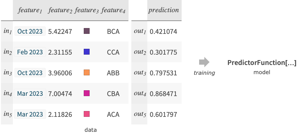
---
title: "Predict"
language: "en"
type: "Symbol"
summary: "Predict[{in1 -> out1, in2 -> out2, ...}] generates a PredictorFunction that attempts to predict outi from the example ini. Predict[data, input] attempts to predict the output associated with input from the training examples given. Predict[data, input, prop] computes the specified property prop relative to the prediction."
keywords: 
- predictor
- regression
- machine learning
- neural networks
- neural nets
- parallel distributed processing
- PDP
- deep belief
- random forest
- nearest neighbors
- probabilistic inference
- statistical inference
- optimization
- probability
- distribution
- conditional distribution
- decision theory
- utility function
- loss function
- artificial intelligence
- learning
- learning theory
- statistical learning
- maximum likelihood
- prior probability
- decision tree
- perceptron
- training
- dataset
- database
- training set
- test set
- validation set
- cross-validation
- feature
- feature vector
- label
- class
- example
- information theory
- bayes theorem
- pattern recognition
- data mining
- data science
- supervised learning
- predictive modeling
- statistical modeling
- predictive analytics
- statistics
canonical_url: "https://reference.wolfram.com/language/ref/Predict.html"
source: "Wolfram Language Documentation"
related_guides: 
  - 
    title: "Machine Learning"
    link: "https://reference.wolfram.com/language/guide/MachineLearning.en.md"
  - 
    title: "Supervised Machine Learning"
    link: "https://reference.wolfram.com/language/guide/SupervisedMachineLearning.en.md"
  - 
    title: "Tabular Modeling"
    link: "https://reference.wolfram.com/language/guide/TabularModeling.en.md"
  - 
    title: "Audio Analysis"
    link: "https://reference.wolfram.com/language/guide/AudioAnalysis.en.md"
  - 
    title: "Scientific Data Analysis"
    link: "https://reference.wolfram.com/language/guide/ScientificDataAnalysis.en.md"
  - 
    title: "Tabular Processing Overview"
    link: "https://reference.wolfram.com/language/guide/TabularProcessing.en.md"
  - 
    title: "Life Sciences & Medicine: Data & Computation"
    link: "https://reference.wolfram.com/language/guide/LifeSciencesAndMedicineDataAndComputation.en.md"
  - 
    title: "Machine Learning Methods"
    link: "https://reference.wolfram.com/language/guide/MachineLearningMethods.en.md"
related_functions: 
  - 
    title: "PredictorFunction"
    link: "https://reference.wolfram.com/language/ref/PredictorFunction.en.md"
  - 
    title: "PredictorMeasurements"
    link: "https://reference.wolfram.com/language/ref/PredictorMeasurements.en.md"
  - 
    title: "Classify"
    link: "https://reference.wolfram.com/language/ref/Classify.en.md"
  - 
    title: "ActivePrediction"
    link: "https://reference.wolfram.com/language/ref/ActivePrediction.en.md"
  - 
    title: "SequencePredict"
    link: "https://reference.wolfram.com/language/ref/SequencePredict.en.md"
  - 
    title: "Interpolation"
    link: "https://reference.wolfram.com/language/ref/Interpolation.en.md"
  - 
    title: "FindFit"
    link: "https://reference.wolfram.com/language/ref/FindFit.en.md"
  - 
    title: "Nearest"
    link: "https://reference.wolfram.com/language/ref/Nearest.en.md"
  - 
    title: "DimensionReduce"
    link: "https://reference.wolfram.com/language/ref/DimensionReduce.en.md"
  - 
    title: "FindFormula"
    link: "https://reference.wolfram.com/language/ref/FindFormula.en.md"
  - 
    title: "BayesianMinimization"
    link: "https://reference.wolfram.com/language/ref/BayesianMinimization.en.md"
---
# Predict

Predict[{in1 -> out1, in2 -> out2, …}] generates a PredictorFunction that attempts to predict outi from the example ini.

Predict[data, input] attempts to predict the output associated with input from the training examples given.

Predict[data, input, prop] computes the specified property prop relative to the prediction.

## Details and Options

* ``Predict`` is used to model the relationship between a scalar variable and examples of many types of data, including numerical, textual, sounds and images.

* This type of modelling, also known as regression analysis, is typically used for tasks like customer behavior analysis, healthcare outcomes prediction, credit risk assessment and more.

[image]

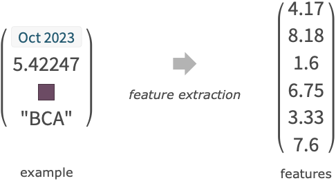
* Complex expressions are automatically converted to simpler features like numbers or classes.

[image]

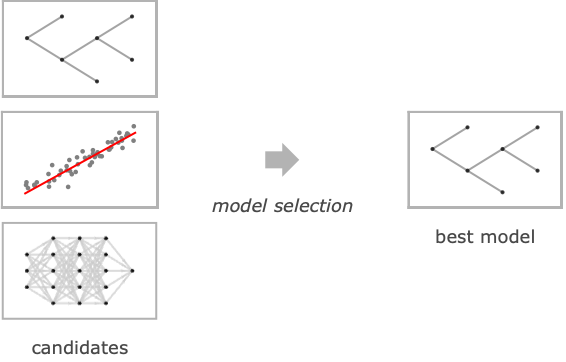
* The final model type and hyperparameter values are selected using cross-validation on the training data.

[image]

* The training ``data`` can have the following structure:

|                                 |                                                      |
| ------------------------------- | ---------------------------------------------------- |
| {in1 -> out1, in2 -> out2, …}     | a list of Rule between input and output              |
| {in1, in2, …} -> {out1, out2, …} | a Rule between inputs and corresponding outputs      |
| {list1, list2, …} -> n           | the nth element of each List as the output           |
| {assoc1, assoc2, …} -> "key"     | the "key" element of each Association as the output  |
| Dataset[…] -> column             | the specified column of Dataset as the output        |
| Tabular[…] -> column             | the specified column of Tabular as the output        |

* In addition, special form of ``data`` include:

|                |                                                      |
| -------------- | ---------------------------------------------------- |
| "name"         | a built-in prediction function                       |
| FittedModel[…] | a fitted model converted into a PredictorFunction[…] |

* Each example input Subscript[in, i] can be a single data element, a list {Subscript[feature, 1], \[Ellipsis]} or an association <\|"Subscript[feature, 1]"->Subscript[value, 1],\[Ellipsis]\|> .

* Each example output ``outi`` must be a numerical value.

* The prediction properties ``prop`` are the same as in ``PredictorFunction``. They include:

|                  |                                                                |
| ---------------- | -------------------------------------------------------------- |
| "Decision"       | best prediction according to distribution and utility function |
| "Distribution"   | distribution of value conditioned on input                     |
| "SHAPValues"     | Shapley additive feature explanations for each example         |
| "SHAPValues" -> n | SHAP explanations using n samples                              |
| "Properties"     | list of all properties available                               |

* ``"SHAPValues"`` assesses the contribution of features by comparing predictions with different sets of features removed and then synthesized. The option ``MissingValueSynthesis`` can be used to specify how the missing features are synthesized. SHAP explanations are given as deviation from the training output mean.

* Examples of built-in predictor functions include:

[`"NameAge"`](https://reference.wolfram.com/language/ref/predictor/NameAge.en.md)	age of a person, given their first name

* The following options can be given:

|                            |           |                                                                   |
| -------------------------- | --------- | ----------------------------------------------------------------- |
| AnomalyDetector            | None      | anomaly detector used by the predictor                            |
| AcceptanceThreshold        | Automatic | rarer probability threshold for anomaly detector                  |
| FeatureExtractor           | Identity  | how to extract features from which to learn                       |
| FeatureNames               | Automatic | feature names to assign for input data                            |
| FeatureTypes               | Automatic | feature types to assume for input data                            |
| IndeterminateThreshold     | 0         | below what probability density to return Indeterminate            |
| Method                     | Automatic | which regression algorithm to use                                 |
| MissingValueSynthesis      | Automatic | how to synthesize missing values                                  |
| PerformanceGoal            | Automatic | aspects of performance to try to optimize                         |
| RecalibrationFunction      | Automatic | how to post-process predicted value                               |
| RandomSeeding              | 1234      | what seeding of pseudorandom generators should be done internally |
| TargetDevice               | "CPU"     | the target device on which to perform training                    |
| TimeGoal                   | Automatic | how long to spend training the classifier                         |
| TrainingProgressReporting  | Automatic | how to report progress during training                            |
| UtilityFunction            | Automatic | utility as function of actual and predicted value                 |
| ValidationSet              | Automatic | data on which to validate the model generated                     |

* Using ``FeatureExtractor -> "Minimal"`` indicates that the internal preprocessing should be as simple as possible.

* Possible settings for ``Method`` include:

|         |                        |                                                                   |
| ------- | ---------------------- | ----------------------------------------------------------------- |
| [image] | "DecisionTree"         | predict using a decision tree                                     |
| [image] | "GradientBoostedTrees" | predict using an ensemble of trees trained with gradient boosting |
| [image] | "LinearRegression"     | predict from linear combinations of features                      |
| [image] | "NearestNeighbors"     | predict from nearest neighboring examples                         |
| [image] | "NeuralNetwork"        | predict using an artificial neural network                        |
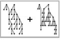
| [image] | "RandomForest"         | predict from Breiman–Cutler ensembles of decision trees           |
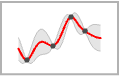
| [image] | "GaussianProcess"      | predict using a Gaussian process prior over functions             |

* Possible settings for ``PerformanceGoal`` include:

|                   |                                                             |
| ----------------- | ----------------------------------------------------------- |
| "DirectTraining"  | train directly on the full dataset, without model searching |
| "Memory"          | minimize storage requirements of the predictor              |
| "Quality"         | maximize accuracy of the predictor                          |
| "Speed"           | maximize speed of the predictor                             |
| "TrainingSpeed"   | minimize time spent producing the predictor                 |
| Automatic         | automatic tradeoff among speed, accuracy and memory         |
| {goal1, goal2, …} | automatically combine goal1, goal2, etc.                    |

* The following settings for ``TrainingProgressReporting`` can be used:

|                     |                                                    |
| ------------------- | -------------------------------------------------- |
| "Panel"             | show a dynamically updating graphical panel        |
| "Print"             | periodically report information using Print        |
| "ProgressIndicator" | show a simple ProgressIndicator                    |
| "SimplePanel"       | dynamically updating panel without learning curves |
| None                | do not report any information                      |

* ``Information`` can be used on the ``PredictorFunction[…]`` obtained.

## Examples (58)

### Basic Examples (2)

Learn to predict the third column of a matrix using the features in the first two columns:

```wl
In[1]:=
p = Predict[(⁠|      |     |      |
| ---- | --- | ---- |
| 1.3  | "P" | 1    |
| 1.8  | "Q" | 2.5  |
| 1.9  | "Q" | 3    |
| 0.2  | "P" | 1    |
| -3.2 | "P" | -4.2 |
| 0.3  | "Q" | 2    |⁠) -> 3]

Out[1]=
PredictorFunction[Association["ExampleNumber" -> 6, 
  "Input" -> Association["Preprocessor" -> MachineLearning`MLProcessor["ToMLDataset", 
      Association["Input" -> Association["f1" -> Association["Type" -> "Numerical"], 
         "f2" -> Assoc ...   "Date" -> DateObject[{2023, 7, 31, 18, 45, 38.932963`8.342892435829247}, "Instant", 
      "Gregorian", 2.], "ProcessorCount" -> 10, "ProcessorType" -> "ARM64", 
    "OperatingSystem" -> "MacOSX", "SystemWordLength" -> 64, "Evaluations" -> {}]]]
```

Predict the value of a new example, given its features:

```wl
In[2]:= p[{1.8, "Q"}]

Out[2]= 0.886385
```

Predict the value of a new example that has a missing feature:

```wl
In[3]:= p[{1.8, Missing[]}]

Out[3]= 0.886385
```

Predict the value of a multiple examples at the same time:

```wl
In[4]:= p[{{1.8, "Q"}, {.4, "P"}}]

Out[4]= {0.886385, 0.881406}
```

---

Train a linear regression on a set of examples:

```wl
In[1]:= data = {1 -> 1.3, 2 -> 2.4, 3 -> 4.4, 4 -> 5.1, 6 -> 7.3};p = Predict[data, Method -> "LinearRegression"]

Out[1]=
PredictorFunction[Association["ExampleNumber" -> 5, 
  "Input" -> Association["Preprocessor" -> MachineLearning`MLProcessor["ToMLDataset", 
      Association["Input" -> Association["f1" -> Association["Type" -> "Numerical"]], 
       "Output" -> As ... te" -> DateObject[{2023, 8, 1, 11, 53, 
       40.708247`8.362257379213888}, "Instant", "Gregorian", 2.], "ProcessorCount" -> 10, 
    "ProcessorType" -> "ARM64", "OperatingSystem" -> "MacOSX", "SystemWordLength" -> 64, 
    "Evaluations" -> {}]]]
```

Get the conditional distribution of the predicted value, given the example feature:

```wl
In[2]:= \[ScriptCapitalD] = p[1.5, "Distribution"]

Out[2]= NormalDistribution[2.03763, 0.375509]
```

Plot the probability density of the distribution:

```wl
In[3]:= Plot[PDF[\[ScriptCapitalD], x], {x, 0, 4}]

Out[3]= [image]
```

Plot the prediction with a confidence band together with the training data:

```wl
In[4]:=
Show[
	ListPlot[List@@@data, PlotStyle -> {Red, PointSize@Large}], 
	ListLinePlot[Table[{x, Around@@p[x, "Distribution"]}, {x, 0, 10}], IntervalMarkers -> "Bands"]
	]

Out[4]= [image]
```

### Scope (24)

#### Data Format (7)

Specify the training set as a list of rules between an input examples and the output value:

```wl
In[1]:= Predict[{1 -> -1.14, 2 -> -0.34, 3 -> 0.46, 4 -> 1.26, 5 -> 2.06}]

Out[1]=
PredictorFunction[Association["ExampleNumber" -> 5, 
  "Input" -> Association["Preprocessor" -> MachineLearning`MLProcessor["ToMLDataset", 
      Association["Input" -> Association["f1" -> Association["Type" -> "Numerical"]], 
       "Output" -> As ... "Date" -> DateObject[{2023, 8, 1, 11, 54, 
       18.2498`8.01383309362523}, "Instant", "Gregorian", 2.], "ProcessorCount" -> 10, 
    "ProcessorType" -> "ARM64", "OperatingSystem" -> "MacOSX", "SystemWordLength" -> 64, 
    "Evaluations" -> {}]]]
```

---

Each example can contain a list of features:

```wl
In[1]:= Predict[{{-0.78, 0.58} -> 0.86, {-0.62, -0.52} -> 2.28, {-0.87, 0.08} -> 1.18, {-0.54, -0.21} -> 2.13, {0.4, -0.58} -> 4.38}]

Out[1]=
PredictorFunction[Association["ExampleNumber" -> 5, 
  "Input" -> Association["Preprocessor" -> MachineLearning`MLProcessor["ToMLDataset", 
      Association["Input" -> Association["f1" -> Association["Type" -> "NumericalVector", 
           "Lengt ...    "Date" -> DateObject[{2023, 8, 1, 11, 54, 19.041385`8.032273518151184}, "Instant", "Gregorian", 
      2.], "ProcessorCount" -> 10, "ProcessorType" -> "ARM64", "OperatingSystem" -> "MacOSX", 
    "SystemWordLength" -> 64, "Evaluations" -> {}]]]
```

---

Each example can contain an association of features:

```wl
In[1]:= Predict[{<|"f1" -> -0.78, "f2" -> 0.58|> -> 0.86, <|"f1" -> -0.62, "f2" -> -0.52|> -> 2.28, <|"f1" -> -0.87, "f2" -> 0.08|> -> 1.18, <|"f1" -> -0.54, "f2" -> -0.21|> -> 2.13, <|"f1" -> 0.4, "f2" -> -0.58|> -> 4.38}]

Out[1]=
PredictorFunction[Association["ExampleNumber" -> 5, 
  "Input" -> Association["Preprocessor" -> MachineLearning`MLProcessor["ToMLDataset", 
      Association["Input" -> Association["f1" -> Association["Type" -> "Numerical"], 
         "f2" -> Assoc ...     "Date" -> DateObject[{2023, 8, 2, 10, 42, 4.069897`7.362158406410211}, "Instant", "Gregorian", 
      2.], "ProcessorCount" -> 10, "ProcessorType" -> "ARM64", "OperatingSystem" -> "MacOSX", 
    "SystemWordLength" -> 64, "Evaluations" -> {}]]]
```

---

Specify the training set a list of rule between a list of input and a list of output:

```wl
In[1]:= Predict[{1, 2, 3, 4, 5} -> {-1.14, -0.34, 0.46, 1.26, 2.06}]

Out[1]=
PredictorFunction[Association["ExampleNumber" -> 5, 
  "Input" -> Association["Preprocessor" -> MachineLearning`MLProcessor["ToMLDataset", 
      Association["Input" -> Association["f1" -> Association["Type" -> "Numerical"]], 
       "Output" -> As ... te" -> DateObject[{2023, 8, 1, 11, 54, 
       19.858041`8.050511387006415}, "Instant", "Gregorian", 2.], "ProcessorCount" -> 10, 
    "ProcessorType" -> "ARM64", "OperatingSystem" -> "MacOSX", "SystemWordLength" -> 64, 
    "Evaluations" -> {}]]]
```

---

Specify all the data in a matrix and mark the output column:

```wl
In[1]:= Predict[{{1, -1.14}, {2, -0.34}, {3, 0.46}, {4, 1.26}, {5, 2.06}} -> 2]

Out[1]=
PredictorFunction[Association["ExampleNumber" -> 5, 
  "Input" -> Association["Preprocessor" -> MachineLearning`MLProcessor["ToMLDataset", 
      Association["Input" -> Association["f1" -> Association["Type" -> "Numerical"]], 
       "Output" -> As ... te" -> DateObject[{2023, 8, 1, 11, 54, 
       20.690806`8.068352392424496}, "Instant", "Gregorian", 2.], "ProcessorCount" -> 10, 
    "ProcessorType" -> "ARM64", "OperatingSystem" -> "MacOSX", "SystemWordLength" -> 64, 
    "Evaluations" -> {}]]]
```

---

Specify all the data in a list of associations and mark the output key:

```wl
In[1]:= Predict[{<|"f1" -> 1, "f2" -> -1.14|>, <|"f1" -> 2, "f2" -> -0.34|>, <|"f1" -> 3, "f2" -> 0.46|>, <|"f1" -> 4, "f2" -> 1.26|>, <|"f1" -> 5, "f2" -> 2.06|>} -> "f2"]

Out[1]=
PredictorFunction[Association["ExampleNumber" -> 5, 
  "Input" -> Association["Preprocessor" -> MachineLearning`MLProcessor["ToMLDataset", 
      Association["Input" -> Association["f1" -> Association["Type" -> "Numerical"]], 
       "Output" -> As ... te" -> DateObject[{2023, 8, 1, 11, 54, 
       21.500033`8.085014109938763}, "Instant", "Gregorian", 2.], "ProcessorCount" -> 10, 
    "ProcessorType" -> "ARM64", "OperatingSystem" -> "MacOSX", "SystemWordLength" -> 64, 
    "Evaluations" -> {}]]]
```

---

Specify all the data in a dataset and mark the output column:

```wl
In[1]:=
Predict[Dataset[{Association["f1" -> 1, "f2" -> -1.1400000000000001], 
  Association["f1" -> 2, "f2" -> -0.34], Association["f1" -> 3, "f2" -> 0.46], 
  Association["f1" -> 4, "f2" -> 1.26], Association["f1" -> 5, "f2" -> 2.06]}] -> "f2"]

Out[1]=
PredictorFunction[Association["ExampleNumber" -> 5, 
  "Input" -> Association["Preprocessor" -> MachineLearning`MLProcessor["ToMLDataset", 
      Association["Input" -> Association["f1" -> Association["Type" -> "Numerical"]], 
       "Output" -> As ... te" -> DateObject[{2023, 8, 1, 11, 54, 
       22.295389`8.100790037287476}, "Instant", "Gregorian", 2.], "ProcessorCount" -> 10, 
    "ProcessorType" -> "ARM64", "OperatingSystem" -> "MacOSX", "SystemWordLength" -> 64, 
    "Evaluations" -> {}]]]
```

#### Data Types (13)

##### Numerical (3)

---

Predict a variable from a number:

```wl
In[1]:= Predict[{0.72 -> -1.56, 0.36 -> -2.28, -0.18 -> -3.36, -0.4 -> -3.8, 0.06 -> -2.88}]

Out[1]=
PredictorFunction[Association["ExampleNumber" -> 5, 
  "Input" -> Association["Preprocessor" -> MachineLearning`MLProcessor["ToMLDataset", 
      Association["Input" -> Association["f1" -> Association["Type" -> "Numerical"]], 
       "Output" -> As ... ate" -> DateObject[{2023, 2, 23, 15, 52, 
       6.333693`7.55423199641137}, "Instant", "Gregorian", 1.], "ProcessorCount" -> 10, 
    "ProcessorType" -> "ARM64", "OperatingSystem" -> "MacOSX", "SystemWordLength" -> 64, 
    "Evaluations" -> {}]]]
```

---

Predict a variable from a numerical vector:

```wl
In[1]:= Predict[{{0.19, 0.44} -> 2.94, {0.82, -0.99} -> 5.63, {-0.82, 0.83} -> 0.53, {-0.25, -0.27} -> 2.77, {-0.9, 0.81} -> 0.39}]

Out[1]=
PredictorFunction[Association["ExampleNumber" -> 5, 
  "Input" -> Association["Preprocessor" -> MachineLearning`MLProcessor["ToMLDataset", 
      Association["Input" -> Association["f1" -> Association["Type" -> "NumericalVector", 
           "Lengt ...  "Date" -> DateObject[{2023, 2, 23, 15, 52, 10.845365`7.7878191591789845}, "Instant", 
      "Gregorian", 1.], "ProcessorCount" -> 10, "ProcessorType" -> "ARM64", 
    "OperatingSystem" -> "MacOSX", "SystemWordLength" -> 64, "Evaluations" -> {}]]]
```

---

Predict a variable from a numerical array or arbitrary depth:

```wl
In[1]:= Predict[{{{0.08, 0.73}, {0.33, -0.45}} -> -0.37, {{0.28, 0.4}, {-0.34, -0.92}} -> -0.64, {{-0.82, 0.35}, {-0.17, 0.93}} -> 0.11, {{0.46, -0.33}, {0.67, 0.82}} -> 1.28, {{0.39, -0.6}, {0.7, 0.34}} -> 0.73}]

Out[1]=
PredictorFunction[Association["ExampleNumber" -> 5, 
  "Input" -> Association["Preprocessor" -> MachineLearning`MLProcessor["ToMLDataset", 
      Association["Input" -> Association["f1" -> Association["Type" -> "NumericalTensor", 
           "Dimen ...   "Date" -> DateObject[{2023, 2, 23, 15, 53, 45.040867`8.406181718624826}, "Instant", 
      "Gregorian", 1.], "ProcessorCount" -> 10, "ProcessorType" -> "ARM64", 
    "OperatingSystem" -> "MacOSX", "SystemWordLength" -> 64, "Evaluations" -> {}]]]
```

##### Nominal (3)

---

Predict a variable from a nominal value:

```wl
In[1]:= Predict[{"B" -> 0.61, "A" -> -0.93, "B" -> 0.26, "B" -> 0.65, "B" -> 0.47}]

Out[1]=
PredictorFunction[Association["ExampleNumber" -> 5, 
  "Input" -> Association["Preprocessor" -> MachineLearning`MLProcessor["ToMLDataset", 
      Association["Input" -> Association["f1" -> Association["Type" -> "Nominal"]], 
       "Output" -> Asso ... ate" -> DateObject[{2023, 8, 1, 11, 55, 
       22.613164`8.10693631558899}, "Instant", "Gregorian", 2.], "ProcessorCount" -> 10, 
    "ProcessorType" -> "ARM64", "OperatingSystem" -> "MacOSX", "SystemWordLength" -> 64, 
    "Evaluations" -> {}]]]
```

---

Predict a variable from several nominal values:

```wl
In[1]:= p = Predict[<|"Treatment" -> {"A", "B", "A", "C", "B", "C", "A", "B", "C", "A"}, "Severity" -> {"High", "Medium", "Low", "High", "Low", "Medium", "Medium", "High", "Low", "High"}, "Recovery Time" -> {8, 6, 4, 9, 5, 7, 6, 8, 5, 8}|> -> "Recovery Time"]

Out[1]=
PredictorFunction[Association["ExampleNumber" -> 10, 
  "Input" -> Association["Preprocessor" -> MachineLearning`MLProcessor["ToMLDataset", 
      Association["Input" -> Association["Treatment" -> Association["Type" -> "Nominal"], 
         "Severi ...    "Date" -> DateObject[{2023, 8, 1, 11, 55, 33.891283`8.282662990108122}, "Instant", "Gregorian", 
      2.], "ProcessorCount" -> 10, "ProcessorType" -> "ARM64", "OperatingSystem" -> "MacOSX", 
    "SystemWordLength" -> 64, "Evaluations" -> {}]]]

In[2]:= p[<|"Treatment" -> "C", "Severity" -> "High"|>]

Out[2]= 9.
```

---

Predict a variable from a mixture of nominal and numerical values:

```wl
In[1]:=
p = Predict[Dataset[{Association["Treatment" -> "A", "Severity" -> "High", "Patient's History" -> "Yes", 
   "Age" -> 55], Association["Treatment" -> "B", "Severity" -> "Medium", 
   "Patient's History" -> "No", "Age" -> 45], Association["Treatment" -> "A", "Severity" -> "Low", 
   "Patient's History" -> "Yes", "Age" -> 30], Association["Treatment" -> "C", 
   "Severity" -> "High", "Patient's History" -> "No", "Age" -> 60], 
  Association["Treatment" -> "B", "Severity" -> "Low", "Patient's History" -> "Yes", "Age" -> 35], 
  Association["Treatment" -> "C", "Severity" -> "Medium", "Patient's History" -> "No", 
   "Age" -> 50]}] -> Dataset[{Association["Recovery Time" -> 8], Association["Recovery Time" -> 6], 
  Association["Recovery Time" -> 4], Association["Recovery Time" -> 9], 
  Association["Recovery Time" -> 5], Association["Recovery Time" -> 7]}]]

Out[1]=
PredictorFunction[Association["ExampleNumber" -> 6, 
  "Input" -> Association["Preprocessor" -> MachineLearning`MLProcessor["ToMLDataset", 
      Association["Input" -> Association["Treatment" -> Association["Type" -> "Nominal"], 
         "Severit ...    "Date" -> DateObject[{2023, 8, 1, 11, 55, 49.474714`8.446958268141286}, "Instant", "Gregorian", 
      2.], "ProcessorCount" -> 10, "ProcessorType" -> "ARM64", "OperatingSystem" -> "MacOSX", 
    "SystemWordLength" -> 64, "Evaluations" -> {}]]]

In[2]:= p[<|"Treatment" -> "C", "Age" -> 42, "Patient's History" -> "No"|>]

Out[2]= 9.
```

##### Quantities (1)

---

Train a predictor on data including ``Quantity`` objects:

```wl
In[1]:=
p = Predict[Dataset[{Association["Neighborhood" -> "Sunnypoint", "Area" -> Quantity[1500, "Feet"^2], 
   "Price" -> Quantity[300000, "USDollars"]], Association["Neighborhood" -> "Moonbrook", 
   "Area" -> Quantity[1800, "Feet"^2], "Price" -> Quantity[360000, "USDollars"]], 
  Association["Neighborhood" -> "Sunnypoint", "Area" -> Quantity[1700, "Feet"^2], 
   "Price" -> Quantity[340000, "USDollars"]], Association["Neighborhood" -> "Starville", 
   "Area" -> Quantity[2000, "Feet"^2], "Price" -> Quantity[500000, "USDollars"]], 
  Association["Neighborhood" -> "Moonbrook", "Area" -> Quantity[1600, "Feet"^2], 
   "Price" -> Quantity[320000, "USDollars"]], Association["Neighborhood" -> "Starville", 
   "Area" -> Quantity[2200, "Feet"^2], "Price" -> Quantity[550000, "USDollars"]], 
  Association["Neighborhood" -> "Sunnypoint", "Area" -> Quantity[1400, "Feet"^2], 
   "Price" -> Quantity[280000, "USDollars"]], Association["Neighborhood" -> "Moonbrook", 
   "Area" -> Quantity[1900, "Feet"^2], "Price" -> Quantity[380000, "USDollars"]], 
  Association["Neighborhood" -> "Starville", "Area" -> Quantity[2100, "Feet"^2], 
   "Price" -> Quantity[520000, "USDollars"]], Association["Neighborhood" -> "Sunnypoint", 
   "Area" -> Quantity[1800, "Feet"^2], "Price" -> Quantity[360000, "USDollars"]]}] -> "Price"]

Out[1]=
PredictorFunction[Association["ExampleNumber" -> 10, 
  "Input" -> Association["Preprocessor" -> MachineLearning`MLProcessor["ToMLDataset", 
      Association["Input" -> Association["Neighborhood" -> Association["Type" -> "Nominal"], 
         "Are ...     "Date" -> DateObject[{2023, 8, 1, 11, 57, 0.596088`6.527885368184133}, "Instant", "Gregorian", 
      2.], "ProcessorCount" -> 10, "ProcessorType" -> "ARM64", "OperatingSystem" -> "MacOSX", 
    "SystemWordLength" -> 64, "Evaluations" -> {}]]]
```

Use the predictor on a new example:

```wl
In[2]:= p[<|"Neighborhood" -> "Moonbrook", "Area" -> Quantity[900, "Feet"^2]|>]

Out[2]= Quantity[279999.9984126983, "USDollars"]
```

Predict the most likely price when only the "Neighborhood" is known:

```wl
In[3]:= p[<|"Neighborhood" -> "Moonbrook"|>]

Out[3]= Quantity[380000.00027971616, "USDollars"]
```

##### Text (1)

---

Get some spam probability data:

```wl
In[1]:=
data = IconizedObject[«spam score»];
First[data]

Out[1]= "Get a free iPhone now!" -> 0.95
```

Train a predictor on the text:

```wl
In[2]:= p = Predict[data]

Out[2]=
PredictorFunction[Association["ExampleNumber" -> 139, 
  "Input" -> Association["Preprocessor" -> MachineLearning`MLProcessor["ToMLDataset", 
      Association["Input" -> Association["f1" -> Association["Type" -> "Text"]], 
       "Output" -> Assoc ...   "Date" -> DateObject[{2025, 6, 11, 11, 18, 48.776661`8.440787043490634}, "Instant", 
      "Gregorian", 2.], "ProcessorCount" -> 10, "ProcessorType" -> "ARM64", 
    "OperatingSystem" -> "MacOSX", "SystemWordLength" -> 64, "Evaluations" -> {}]]]
```

Use the predictor on new examples:

```wl
In[3]:= p[{"Monday meeting rescheduled", "You have won a yacht!"}]

Out[3]= {0.0857944, 0.86061}
```

##### Colors (1)

---

Predict a variable from a color expression:

```wl
In[1]:= Predict[{RGBColor[0.374533954339318, 0.07318946913456625, 0.34948076712998266], RGBColor[0.7085138807325013, 0.5508514126801727, 0.270668676806443], RGBColor[0.482424250096966, 0.9866683639813978, 0.8763664701273515], RGBColor[0.9143901752719417, 0.5933340939498908, 0.12490074751913904], RGBColor[0.5435848746538026, 0.3320246736743131, 0.10546267186910474], RGBColor[0.4838618865454345, 0.1408408308353548, 0.4182003855819225], RGBColor[0.09486596097451105, 0.4061453278622089, 0.19070989282627604], RGBColor[0.9978640282936782, 0.9850053326406092, 0.6079629315168287], RGBColor[0.7423358808871543, 0.14441876671667964, 0.44156741749306994], RGBColor[0.11647231911978806, 0.14156287966553882, 0.7585884183769138], RGBColor[0.413441306192059, 0.35488417001075656, 0.4547933589911124], RGBColor[0.6479088100736257, 0.06575533518383936, 0.33956768046537045], RGBColor[0.43617515288692754, 0.395321922119783, 0.03284974966398546], RGBColor[0.08988572988782773, 0.45387554090065807, 0.565445988533821], RGBColor[0.5962404964416488, 0.7115775209469246, 0.5937470103610984], RGBColor[0.5425615924830165, 0.9052557429558079, 0.7950524706591187], RGBColor[0.258709017611374, 0.05898221147135585, 0.04550888101080042], RGBColor[0.733150150511475, 0.5972827779202361, 0.34440914488265517], RGBColor[0.9604086664357256, 0.9762505577301217, 0.6004232657263842], RGBColor[0.10316670441111997, 0.3667737206326349, 0.46355431351130827]} -> {0.22, 0.61, 0.91, 0.7, 0.42, 0.31, 0.38, 0.97, 0.44, 0.26, 0.41, 0.37, 0.43, 0.45, 0.71, 0.85, 0.13, 0.65, 0.96, 0.37}, {Red, Green, Blue}]

Out[1]= {0.333485, 0.653957, 0.188904}
```

##### Images (1)

---

Train a predictor to predict the colored area of an image:

```wl
In[1]:= Predict[{[image] -> 40.2, [image] -> 8.9, [image] -> 11., [image] -> 4.9, [image] -> 13.6, [image] -> 15.6, [image] -> 14.7, [image] -> 3.8, [image] -> 34.7, [image] -> 10.8, [image] -> 4., [image] -> 16.1, [image] -> 3.3, [image] -> 8.3, [image] -> 12.6}]

Out[1]= PredictorFunction[«1»]
```

##### Sequences (1)

---

Train a predictor on data where the feature is a sequence of tokens:

```wl
In[1]:= Predict[{{"butter", "sugar", "flour"} -> 0.2, {"flour", "butter"} -> 1.4, {"tomato", "salt"} -> 0.9}]

Out[1]=
PredictorFunction[Association["ExampleNumber" -> 3, 
  "Input" -> Association["Preprocessor" -> MachineLearning`MLProcessor["ToMLDataset", 
      Association["Input" -> Association["f1" -> Association["Type" -> "NominalSequence"]], 
       "Output" ...  "Date" -> DateObject[{2018, 11, 29, 21, 4, 59.808326`8.529336620001672}, "Instant", 
      "Gregorian", -8.], "ProcessorCount" -> 4, "ProcessorType" -> "x86-64", 
    "OperatingSystem" -> "MacOSX", "SystemWordLength" -> 64, "Evaluations" -> {}]]]
```

##### Missing Data (2)

---

Train on a dataset containing missing features:

```wl
In[1]:= Predict[{{2.3, "male"} -> 1, {4.8, Missing[]} -> 2.5, {Missing[], "female"} -> 8.4, {5.2, "female"} -> -2, {Missing[], "male"} -> -4.2, {1.3, "male"} -> 10}]

Out[1]=
PredictorFunction[Association["ExampleNumber" -> 6, 
  "Input" -> Association["Preprocessor" -> MachineLearning`MLProcessor["ToMLDataset", 
      Association["Input" -> Association["f1" -> Association["Type" -> "Numerical"], 
         "f2" -> Assoc ... e" -> DateObject[{2023, 11, 6, 16, 21, 
       48.244932`8.436026674679537}, "Instant", "Gregorian", 1.], "ProcessorCount" -> 10, 
    "ProcessorType" -> "ARM64", "OperatingSystem" -> "MacOSX", "SystemWordLength" -> 64, 
    "Evaluations" -> {}]]]
```

---

Train a predictor on a dataset with named features. The order of the keys does not matter. Keys can be missing:

```wl
In[1]:=
p = Predict[{
	<|"age" -> 24, "sex" -> "female"|> -> 10.4, 
	<|"sex" -> "male", "age" -> 13|> -> 5.2, 
	<|"age" -> 57|> -> 23.3, 
	<|"sex" -> "male"|> -> 14.3}]

Out[1]=
PredictorFunction[Association["ExampleNumber" -> 4, 
  "Input" -> Association["Preprocessor" -> MachineLearning`MLProcessor["ToMLDataset", 
      Association["Input" -> Association["age" -> Association["Type" -> "Numerical"], 
         "sex" -> Ass ...    "Date" -> DateObject[{2023, 11, 6, 16, 21, 50.63849`8.457055722404327}, "Instant", "Gregorian", 
      1.], "ProcessorCount" -> 10, "ProcessorType" -> "ARM64", "OperatingSystem" -> "MacOSX", 
    "SystemWordLength" -> 64, "Evaluations" -> {}]]]
```

Predict examples containing missing features:

```wl
In[2]:= p[{<|"age" -> 31|>, <|"sex" -> "male"|>, <||>}]

Out[2]= {12.3714, 11.3255, 12.5104}
```

#### Information (4)

Extract information from a trained predictor:

```wl
In[1]:=
Information[PredictorFunction[Association["ExampleNumber" -> 6, 
  "Input" -> Association["Preprocessor" -> MachineLearning`MLProcessor["ToMLDataset", 
      Association["Input" -> Association["f1" -> Association["Type" -> "Numerical"], 
         "f2" -> Assoc ...   "Date" -> DateObject[{2023, 7, 26, 16, 30, 52.286118`8.470961373666972}, "Instant", 
      "Gregorian", 2.], "ProcessorCount" -> 10, "ProcessorType" -> "ARM64", 
    "OperatingSystem" -> "MacOSX", "SystemWordLength" -> 64, "Evaluations" -> {}]]]]

Out[1]=
MachineLearning`MLInformationObject[PredictorFunction[Association["ExampleNumber" -> 6, 
   "Input" -> Association["Preprocessor" -> MachineLearning`MLProcessor["ToMLDataset", 
       Association["Input" -> Association["f1" -> Association["Type" -> ... Date" -> DateObject[{2023, 7, 26, 16, 30, 52.286118`8.470961373666972}, "Instant", 
       "Gregorian", 2.], "ProcessorCount" -> 10, "ProcessorType" -> "ARM64", 
     "OperatingSystem" -> "MacOSX", "SystemWordLength" -> 64, "Evaluations" -> {}]]]]
```

---

Get information about the input features:

```wl
In[1]:=
Information[PredictorFunction[Association["ExampleNumber" -> 6, 
  "Input" -> Association["Preprocessor" -> MachineLearning`MLProcessor["ToMLDataset", 
      Association["Input" -> Association["f1" -> Association["Type" -> "Numerical"], 
         "f2" -> Assoc ...   "Date" -> DateObject[{2023, 7, 26, 16, 30, 52.286118`8.470961373666972}, "Instant", 
      "Gregorian", 2.], "ProcessorCount" -> 10, "ProcessorType" -> "ARM64", 
    "OperatingSystem" -> "MacOSX", "SystemWordLength" -> 64, "Evaluations" -> {}]]], #]& /@ {"FeatureNames", "FeatureNumber", "FeatureTypes"}

Out[1]= {{"f1", "f2"}, 2, <|"f1" -> "Numerical", "f2" -> "Nominal"|>}
```

---

Get the feature extractor used to process the input features:

```wl
In[1]:=
Information[PredictorFunction[Association["ExampleNumber" -> 6, 
  "Input" -> Association["Preprocessor" -> MachineLearning`MLProcessor["ToMLDataset", 
      Association["Input" -> Association["f1" -> Association["Type" -> "Numerical"], 
         "f2" -> Assoc ...   "Date" -> DateObject[{2023, 7, 26, 16, 30, 52.286118`8.470961373666972}, "Instant", 
      "Gregorian", 2.], "ProcessorCount" -> 10, "ProcessorType" -> "ARM64", 
    "OperatingSystem" -> "MacOSX", "SystemWordLength" -> 64, "Evaluations" -> {}]]], "FeatureExtractor"]

Out[1]=
FeatureExtractorFunction[Association["ExampleNumber" -> 6, 
  "Preprocessor" -> MachineLearning`MLProcessor["ToMLDataset", 
    Association["Input" -> Association["f1" -> Association["Type" -> "Numerical"], 
       "f2" -> Association["Type" -> "No ... on" -> {13.4, 0}, 
    "Date" -> DateObject[{2023, 7, 26, 16, 31, 38.768742`8.341056687686939}, "Instant", 
      "Gregorian", 2.], "ProcessorCount" -> 10, "ProcessorType" -> "ARM64", 
    "OperatingSystem" -> "MacOSX", "SystemWordLength" -> 64]]]
```

---

Get a list of the supported properties

```wl
In[1]:=
Information[PredictorFunction[Association["ExampleNumber" -> 6, 
  "Input" -> Association["Preprocessor" -> MachineLearning`MLProcessor["ToMLDataset", 
      Association["Input" -> Association["f1" -> Association["Type" -> "Numerical"], 
         "f2" -> Assoc ...   "Date" -> DateObject[{2023, 7, 26, 16, 30, 52.286118`8.470961373666972}, "Instant", 
      "Gregorian", 2.], "ProcessorCount" -> 10, "ProcessorType" -> "ARM64", 
    "OperatingSystem" -> "MacOSX", "SystemWordLength" -> 64, "Evaluations" -> {}]]], "Properties"]

Out[1]= {"AcceptanceThreshold", "AnomalyDetector", "BatchEvaluationSpeed", "BatchEvaluationTime", "Calibrated", "EvaluationTime", "ExampleNumber", "FeatureExtractor", "FeatureNames", "FeatureNumber", "FeatureTypes", "FunctionMemory", "FunctionProperties",  ... Curve", "MaxTrainingMemory", "MeanCrossEntropy", "Method", "MethodDescription", "MethodOption", "MethodParameters", "MissingSynthesizer", "PerformanceGoal", "Properties", "StandardDeviation", "TrainingLabelMean", "TrainingTime", "UtilityFunction"}
```

### Options (23)

#### AcceptanceThreshold (1)

Create a predictor with an anomaly detector:

```wl
In[1]:= p = Predict[{1 -> 1.2, 2 -> 3.5, 3.5 -> 5.4, 4 -> 2.3}, AnomalyDetector -> Automatic]

Out[1]= PredictorFunction[…]
```

Change the value of the acceptance threshold when evaluating the predictor:

```wl
In[2]:= p[6, AcceptanceThreshold -> 0.01]

Out[2]= Missing["Anomalous"]

In[3]:= p[6, AcceptanceThreshold -> 0.0001]

Out[3]= 3.85
```

Permanently change the value of the acceptance threshold in the predictor:

```wl
In[4]:= p2 = Predict[p, AcceptanceThreshold -> 0.01]

Out[4]= PredictorFunction[…]

In[5]:= p2[6]

Out[5]= Missing["Anomalous"]
```

#### AnomalyDetector (1)

Create a predictor and specify that an anomaly detector should be included:

```wl
In[1]:= p = Predict[{1 -> 1.2, 2 -> 3.5, 3.5 -> 5.4, 4 -> 2.3}, AnomalyDetector -> Automatic]

Out[1]= PredictorFunction[…]
```

Evaluate the predictor on a non-anomalous input:

```wl
In[2]:= p[1.2]

Out[2]= 2.35
```

Evaluate the predictor on an anomalous input:

```wl
In[3]:= p[100000.2]

Out[3]= Missing["Anomalous"]
```

The ``"Distribution"`` property is not affected by the anomaly detector:

```wl
In[4]:= p[100000.2, "Distribution"]

Out[4]= NormalDistribution[3.85, 2.23448]
```

Temporarily remove the anomaly detector from the predictor:

```wl
In[5]:= p[10000.2, AnomalyDetector -> None]

Out[5]= 3.85
```

Permanently remove the anomaly detector from the predictor:

```wl
In[6]:= p2 = Predict[p, AnomalyDetector -> None]

Out[6]= PredictorFunction[…]

In[7]:= p2[10000.2]

Out[7]= 3.85
```

#### FeatureExtractor (2)

Generate a predictor function using ``FeatureExtractor`` to preprocess the data using a custom function:

```wl
In[1]:= data = {DateObject[{2014, 5, 5}, TimeObject[{9, 53, 6.30158}, TimeZone -> -5.], TimeZone -> -5.] -> 1, DateObject[{2000, 1, 1}, TimeObject[{0, 0, 0.}, TimeZone -> -5.], TimeZone -> -5.] -> 2, DateObject[{2007, 8, 23}] -> 3, DateObject[{2016, 4, 4}, TimeObject[{15, 59, 18.2738}, TimeZone -> -4.], TimeZone -> -4.] -> 4};

In[2]:= p = Predict[data, FeatureExtractor -> ({AbsoluteTime[#], #["Year"]}&)]

Out[2]=
PredictorFunction[Association["ExampleNumber" -> 4, 
  "Input" -> Association["Preprocessor" -> MachineLearning`MLProcessor["ToMLDataset", 
      Association["Input" -> Association["f1" -> Association["Type" -> "Date"]], 
       "Output" -> Associa ...   "Date" -> DateObject[{2018, 11, 29, 21, 7, 5.119861`7.461833158195371}, "Instant", "Gregorian", 
      -8.], "ProcessorCount" -> 4, "ProcessorType" -> "x86-64", "OperatingSystem" -> "MacOSX", 
    "SystemWordLength" -> 64, "Evaluations" -> {}]]]
```

Add the ``"StandardizedVector"`` method to the preprocessing pipeline:

```wl
In[3]:= p = Predict[data, FeatureExtractor -> {{AbsoluteTime[#], #["Year"]}&, "StandardizedVector"}]

Out[3]=
PredictorFunction[Association["ExampleNumber" -> 4, 
  "Input" -> Association["Preprocessor" -> MachineLearning`MLProcessor["ToMLDataset", 
      Association["Input" -> Association["f1" -> Association["Type" -> "Date"]], 
       "Output" -> Associa ...   "Date" -> DateObject[{2018, 11, 29, 21, 7, 9.982093`7.751796598438311}, "Instant", "Gregorian", 
      -8.], "ProcessorCount" -> 4, "ProcessorType" -> "x86-64", "OperatingSystem" -> "MacOSX", 
    "SystemWordLength" -> 64, "Evaluations" -> {}]]]
```

Use the predictor on new data:

```wl
In[4]:= p[DateObject[{2017, 1, 18}, TimeObject[{23, 24, 10.099}, TimeZone -> -5.], TimeZone -> -5.]]

Out[4]= 2.721
```

---

Create a feature extractor and extract features from a dataset:

```wl
In[1]:= {features, fe} = FeatureExtraction[{DateObject[{2014, 5, 5, 9, 53, 6.30158}, "Instant", "Gregorian", -5.], DateObject[{2000, 1, 1, 0, 0, 0.}, "Instant", "Gregorian", -5.], DateObject[{2007, 8, 23}, "Day", "Gregorian", -5.], DateObject[{2016, 4, 4, 15, 59, 18.2738}, "Instant", "Gregorian", -4.]}, {{AbsoluteTime[#], #["Year"]}&, "StandardizedVector"}, {"ExtractedFeatures", "ExtractorFunction"}]

Out[1]=
{{{0.749429, 0.753992}, {-1.49852, -1.4683}, {-0.300822, -0.357154}, {1.04991, 1.07146}}, FeatureExtractorFunction[Association["ExampleNumber" -> 4, 
  "Preprocessor" -> MachineLearning`MLProcessor["ToMLDataset", 
    Association["Input" -> Associa ...  -> DateObject[{2018, 11, 29, 21, 7, 
       18.006644`8.008007762694954}, "Instant", "Gregorian", -8.], "ProcessorCount" -> 4, 
    "ProcessorType" -> "x86-64", "OperatingSystem" -> "MacOSX", "SystemWordLength" -> 64, 
    "Evaluations" -> {}]]]}
```

Train a predictor on the extracted features:

```wl
In[2]:= p = Predict[features -> {1, 2, 3, 4}]

Out[2]=
PredictorFunction[Association["ExampleNumber" -> 4, 
  "Input" -> Association["Preprocessor" -> MachineLearning`MLProcessor["ToMLDataset", 
      Association["Input" -> Association["f1" -> Association["Type" -> "NumericalVector", 
           "Lengt ...  "Date" -> DateObject[{2018, 11, 29, 21, 7, 21.580983`8.086646206066002}, "Instant", 
      "Gregorian", -8.], "ProcessorCount" -> 4, "ProcessorType" -> "x86-64", 
    "OperatingSystem" -> "MacOSX", "SystemWordLength" -> 64, "Evaluations" -> {}]]]
```

Join the feature extractor to the predictor:

```wl
In[3]:= p2 = Predict[p, FeatureExtractor -> fe]

Out[3]=
PredictorFunction[Association["ExampleNumber" -> 4, 
  "Input" -> Association["Preprocessor" -> MachineLearning`MLProcessor["ToMLDataset", 
      Association["Input" -> Association["f1" -> Association["Type" -> "Date"]], 
       "Output" -> Associa ...  "Date" -> DateObject[{2018, 11, 29, 21, 7, 21.580983`8.086646206066002}, "Instant", 
      "Gregorian", -8.], "ProcessorCount" -> 4, "ProcessorType" -> "x86-64", 
    "OperatingSystem" -> "MacOSX", "SystemWordLength" -> 64, "Evaluations" -> {}]]]
```

The predictor can now be used on the initial input type:

```wl
In[4]:= p2[DateObject[{2017, 1, 18}, TimeObject[{23, 24, 10.099}, TimeZone -> -5.], TimeZone -> -5.]]

Out[4]= 2.72107
```

#### FeatureNames (2)

Train a predictor and give a name to each feature:

```wl
In[1]:= p = Predict[{{2.3, "male"} -> 1, {4.8, Missing[]} -> 2.5, {Missing[], "female"} -> 8.4, {5.2, "female"} -> -2, {Missing[], "male"} -> -4.2, {1.3, "male"} -> 10}, FeatureNames -> {"age", "gender"}]

Out[1]=
PredictorFunction[Association["ExampleNumber" -> 6, 
  "Input" -> Association["Preprocessor" -> MachineLearning`MLProcessor["ToMLDataset", 
      Association["Input" -> Association["age" -> Association["Type" -> "Numerical"], 
         "gender" ->  ... " -> DateObject[{2018, 11, 29, 21, 7, 
       34.243672`8.287155308433288}, "Instant", "Gregorian", -8.], "ProcessorCount" -> 4, 
    "ProcessorType" -> "x86-64", "OperatingSystem" -> "MacOSX", "SystemWordLength" -> 64, 
    "Evaluations" -> {}]]]
```

Use the association format to predict a new example:

```wl
In[2]:= p[<|"age" -> 3.3, "gender" -> "male"|>]

Out[2]= 2.61667
```

The list format can still be used:

```wl
In[3]:= p[{3.3, "male"}]

Out[3]= 2.61667
```

---

Train a predictor on a training set with named features and use ``FeatureNames`` to set their order:

```wl
In[1]:= p = Predict[{<|"age" -> 2.3, "gender" -> "male"|> -> 1, <|"age" -> 4.6|> -> 2.5, <|"gender" -> "female"|> -> 8.4, <|"gender" -> "female", "age" -> 5.2|> -> -2}, FeatureNames -> {"gender", "age"}]

Out[1]=
PredictorFunction[Association["ExampleNumber" -> 4, 
  "Input" -> Association["Preprocessor" -> MachineLearning`MLProcessor["ToMLDataset", 
      Association["Input" -> Association["gender" -> Association["Type" -> "Nominal"], 
         "age" -> As ...   "Date" -> DateObject[{2018, 11, 29, 21, 7, 43.207757`8.38813669924369}, "Instant", "Gregorian", 
      -8.], "ProcessorCount" -> 4, "ProcessorType" -> "x86-64", "OperatingSystem" -> "MacOSX", 
    "SystemWordLength" -> 64, "Evaluations" -> {}]]]
```

Features are ordered as specified:

```wl
In[2]:= Information[p, FeatureNames]

Out[2]= {"gender", "age"}
```

Predict a new example from a list:

```wl
In[3]:= p[{"female", 6.5}]

Out[3]= 3.2
```

#### FeatureTypes (2)

Train a predictor on textual and nominal data:

```wl
In[1]:= trainingset = {{"example", "a"} -> 1.4, {"example", "a"} -> 2.7, {"an example again", "b"} -> 2.7};

In[2]:= p = Predict[trainingset]

Out[2]=
PredictorFunction[Association["ExampleNumber" -> 3, 
  "Input" -> Association["Preprocessor" -> MachineLearning`MLProcessor["ToMLDataset", 
      Association["Input" -> Association["f1" -> Association["Type" -> "Nominal"], 
         "f2" -> Associa ...    "Date" -> DateObject[{2023, 7, 26, 19, 1, 13.180773`7.872515866265958}, "Instant", "Gregorian", 
      2.], "ProcessorCount" -> 10, "ProcessorType" -> "ARM64", "OperatingSystem" -> "MacOSX", 
    "SystemWordLength" -> 64, "Evaluations" -> {}]]]
```

The first feature has been wrongly interpreted as a nominal feature:

```wl
In[3]:= Information[p, FeatureTypes]

Out[3]= <|"f1" -> "Nominal", "f2" -> "Nominal"|>
```

Specify that the first feature should be considered textual:

```wl
In[4]:= p = Predict[trainingset, FeatureTypes -> {"Text", "Nominal"}]

Out[4]=
PredictorFunction[Association["ExampleNumber" -> 3, 
  "Input" -> Association["Preprocessor" -> MachineLearning`MLProcessor["ToMLDataset", 
      Association["Input" -> Association["f1" -> Association["Type" -> "Text"], 
         "f2" -> Associatio ...    "Date" -> DateObject[{2023, 7, 26, 19, 1, 16.257608`7.963631632522637}, "Instant", "Gregorian", 
      2.], "ProcessorCount" -> 10, "ProcessorType" -> "ARM64", "OperatingSystem" -> "MacOSX", 
    "SystemWordLength" -> 64, "Evaluations" -> {}]]]

In[5]:= Information[p, FeatureTypes]

Out[5]= <|"f1" -> "Text", "f2" -> "Nominal"|>
```

Predict a new example:

```wl
In[6]:= p[{"a new example", "b"}]

Out[6]= 2.26692
```

---

Train a predictor with named features:

```wl
In[1]:=
trainingset = {
	<|"age" -> 32, "gender" -> 1|> -> 4.3, 
	<|"age" -> 41, "gender" -> 2|> -> 1.2, 
	<|"age" -> 17, "gender" -> 2|> -> 1.4, 
	<|"age" -> 11, "gender" -> 1|> -> 5.1};

In[2]:= p = Predict[trainingset]

Out[2]=
PredictorFunction[Association["ExampleNumber" -> 4, 
  "Input" -> Association["Preprocessor" -> MachineLearning`MLProcessor["ToMLDataset", 
      Association["Input" -> Association["age" -> Association["Type" -> "Numerical"], 
         "gender" ->  ...  "Date" -> DateObject[{2018, 12, 2, 18, 55, 17.087302`7.985248479718306}, "Instant", 
      "Gregorian", -5.], "ProcessorCount" -> 4, "ProcessorType" -> "x86-64", 
    "OperatingSystem" -> "MacOSX", "SystemWordLength" -> 64, "Evaluations" -> {}]]]
```

Both features have been considered numerical:

```wl
In[3]:= Information[p, FeatureTypes]

Out[3]= <|"age" -> "Numerical", "gender" -> "Numerical"|>
```

Specify that the feature "gender" should be considered nominal:

```wl
In[4]:= p = Predict[trainingset, FeatureTypes -> <|"gender" -> "Nominal"|>]

Out[4]=
PredictorFunction[Association["ExampleNumber" -> 4, 
  "Input" -> Association["Preprocessor" -> MachineLearning`MLProcessor["ToMLDataset", 
      Association["Input" -> Association["age" -> Association["Type" -> "Numerical"], 
         "gender" ->  ...   "Date" -> DateObject[{2018, 12, 2, 18, 55, 20.47686`8.063838344737976}, "Instant", "Gregorian", 
      -5.], "ProcessorCount" -> 4, "ProcessorType" -> "x86-64", "OperatingSystem" -> "MacOSX", 
    "SystemWordLength" -> 64, "Evaluations" -> {}]]]

In[5]:= Information[p, FeatureTypes]

Out[5]= <|"age" -> "Numerical", "gender" -> "Nominal"|>
```

#### IndeterminateThreshold (1)

Specify a probability density threshold when training the predictor:

```wl
In[1]:= p = Predict[{1 -> 1.2, 2 -> 1.4, 3 -> 4.5, 4 -> 6.8}, IndeterminateThreshold -> 0.5]

Out[1]=
PredictorFunction[Association["ExampleNumber" -> 4, 
  "Input" -> Association["Preprocessor" -> MachineLearning`MLProcessor["ToMLDataset", 
      Association["Input" -> Association["f1" -> Association["Type" -> "Numerical"]], 
       "Output" -> As ... " -> DateObject[{2018, 12, 2, 18, 55, 
       32.487449`8.264290591169907}, "Instant", "Gregorian", -5.], "ProcessorCount" -> 4, 
    "ProcessorType" -> "x86-64", "OperatingSystem" -> "MacOSX", "SystemWordLength" -> 64, 
    "Evaluations" -> {}]]]
```

Visualize the probability density for a given example:

```wl
In[2]:=
example = 3.4;
pdf = PDF[p[example, "Distribution"]]

Out[2]= Function[\[FormalX], 0.422198 E^-0.559992 (-5.26222 + \[FormalX])^2]

In[3]:= Plot[pdf[x], {x, 2, 8}, PlotRange -> All]

Out[3]= [image]
```

As no value has a probability density above 0.5, no prediction is made:

```wl
In[4]:= p[example]

Out[4]= Indeterminate
```

Specifying a threshold when predicting supersedes the trained threshold:

```wl
In[5]:= p[example, IndeterminateThreshold -> 0.]

Out[5]= 5.26222
```

Update the value of the threshold in the predictor:

```wl
In[6]:= p2 = Predict[p, IndeterminateThreshold -> 0.]

Out[6]=
PredictorFunction[Association["ExampleNumber" -> 4, 
  "Input" -> Association["Preprocessor" -> MachineLearning`MLProcessor["ToMLDataset", 
      Association["Input" -> Association["f1" -> Association["Type" -> "Numerical"]], 
       "Output" -> As ... " -> DateObject[{2018, 12, 2, 18, 55, 
       32.487449`8.264290591169907}, "Instant", "Gregorian", -5.], "ProcessorCount" -> 4, 
    "ProcessorType" -> "x86-64", "OperatingSystem" -> "MacOSX", "SystemWordLength" -> 64, 
    "Evaluations" -> {}]]]

In[7]:= p2[example]

Out[7]= 5.26222
```

#### Method (4)

Train a linear predictor:

```wl
In[1]:= trainingset = {1, 2, 3, 4, 5, 6} -> {2, 3, 5, 8, 9, 7};

In[2]:= linear = Predict[trainingset, Method -> "LinearRegression"]

Out[2]=
PredictorFunction[Association["ExampleNumber" -> 6, 
  "Input" -> Association["Preprocessor" -> MachineLearning`MLProcessor["ToMLDataset", 
      Association["Input" -> Association["f1" -> Association["Type" -> "Numerical"]], 
       "Output" -> As ... te" -> DateObject[{2023, 7, 26, 17, 32, 
       4.983533`7.450112326490211}, "Instant", "Gregorian", 2.], "ProcessorCount" -> 10, 
    "ProcessorType" -> "ARM64", "OperatingSystem" -> "MacOSX", "SystemWordLength" -> 64, 
    "Evaluations" -> {}]]]
```

Train a nearest-neighbors predictor:

```wl
In[3]:= nn = Predict[trainingset, Method -> "NearestNeighbors"]

Out[3]=
PredictorFunction[Association["ExampleNumber" -> 6, 
  "Input" -> Association["Preprocessor" -> MachineLearning`MLProcessor["ToMLDataset", 
      Association["Input" -> Association["f1" -> Association["Type" -> "Numerical"]], 
       "Output" -> As ... ate" -> DateObject[{2023, 7, 26, 17, 32, 
       5.087543`7.45908308070933}, "Instant", "Gregorian", 2.], "ProcessorCount" -> 10, 
    "ProcessorType" -> "ARM64", "OperatingSystem" -> "MacOSX", "SystemWordLength" -> 64, 
    "Evaluations" -> {}]]]
```

Plot the predicted value as a function of the feature for both predictors:

```wl
In[4]:= Plot[{linear[x], nn[x]}, {x, 0, 7}, Exclusions -> None]

Out[4]= [image]
```

---

Train a random forest predictor:

```wl
In[1]:= trainingset = ExampleData[{"MachineLearning", "BostonHomes"}, "TrainingData"];

In[2]:= p1 = Predict[trainingset, Method -> "RandomForest"]

Out[2]= PredictorFunction[«1»]
```

Find the standard deviation of the residuals on a test set:

```wl
In[3]:= testset = ExampleData[{"MachineLearning", "BostonHomes"}, "TestData"];

In[4]:= PredictorMeasurements[p1, testset, "StandardDeviation"]

Out[4]= 4.91105
```

In this example, using a linear regression predictor increases the standard deviation of the residuals:

```wl
In[5]:= p2 = Predict[trainingset, Method -> "LinearRegression"]

Out[5]=
PredictorFunction[Association["ExampleNumber" -> 338, 
  "Input" -> Association["Preprocessor" -> MachineLearning`MLProcessor["ToMLDataset", 
      Association["Input" -> Association["f1" -> Association["Type" -> "Numerical"], 
         "f2" -> Ass ... " -> DateObject[{2018, 11, 30, 7, 17, 
       56.975398`8.508262341500377}, "Instant", "Gregorian", -8.], "ProcessorCount" -> 4, 
    "ProcessorType" -> "x86-64", "OperatingSystem" -> "MacOSX", "SystemWordLength" -> 64, 
    "Evaluations" -> {}]]]

In[6]:= PredictorMeasurements[p2, testset, "StandardDeviation"]

Out[6]= 5.7013
```

However, using a linear regression predictor reduces the training time:

```wl
In[7]:= Information[#, "TrainingTime"] & /@ {p1, p2}

Out[7]= {Quantity[0.499554, "Seconds"], Quantity[1.400285, "Seconds"]}
```

---

Train a linear regression, neural network, and Gaussian process predictor:

```wl
In[1]:= data = {1, 2, 3, 4, 5, 6, 7, 8, 9} -> {1, 2, 3, 4, 5, 6, 7, 8, 9} ^ 4;

In[2]:= {neural, linear, gaussprocess} = Predict[data, Method -> #]& /@ {"NeuralNetwork", "LinearRegression", "GaussianProcess"}

Out[2]=
{PredictorFunction[Association["ExampleNumber" -> 9, 
  "Input" -> Association["Preprocessor" -> MachineLearning`MLProcessor["ToMLDataset", 
      Association["Input" -> Association["f1" -> Association["Type" -> "Numerical"]], 
       "Output" -> A ... " -> DateObject[{2023, 7, 26, 17, 33, 
       0.384639`6.3376283060517205}, "Instant", "Gregorian", 2.], "ProcessorCount" -> 10, 
    "ProcessorType" -> "ARM64", "OperatingSystem" -> "MacOSX", "SystemWordLength" -> 64, 
    "Evaluations" -> {}]]]}
```

These methods produce smooth predictors:

```wl
In[3]:= Show[ListPlot@data[[2]], Plot[{neural[x], linear[x], gaussprocess[x]}, {x, 0, 10}, Exclusions -> None]]

Out[3]= [image]
```

Train a random forest and nearest-neighbor predictor:

```wl
In[4]:= {nearest, forest} = Predict[data, Method -> #]& /@ {"NearestNeighbors", "RandomForest"}

Out[4]=
{PredictorFunction[Association["ExampleNumber" -> 9, 
  "Input" -> Association["Preprocessor" -> MachineLearning`MLProcessor["ToMLDataset", 
      Association["Input" -> Association["f1" -> Association["Type" -> "Numerical"]], 
       "Output" -> A ... e" -> DateObject[{2023, 7, 26, 17, 33, 
       15.890212`7.95370467647465}, "Instant", "Gregorian", 2.], "ProcessorCount" -> 10, 
    "ProcessorType" -> "ARM64", "OperatingSystem" -> "MacOSX", "SystemWordLength" -> 64, 
    "Evaluations" -> {}]]]}
```

These methods produce non-smooth predictors:

```wl
In[5]:= Show[ListPlot@data[[2]], Plot[{forest[x], nearest[x]}, {x, 0, 10}, Exclusions -> None]]

Out[5]= [image]
```

---

Train a neural network, a random forest, and a Gaussian process predictor:

```wl
In[1]:= data = Table[n -> Sin[n], {n, 1, 10}];

In[2]:= {neuralnetwork, randomforest, gaussianprocess} = Predict[data, Method -> #]& /@ {"NeuralNetwork", "RandomForest", "GaussianProcess"}

Out[2]=
{PredictorFunction[Association["ExampleNumber" -> 10, 
  "Input" -> Association["Preprocessor" -> MachineLearning`MLProcessor["ToMLDataset", 
      Association["Input" -> Association["f1" -> Association["Type" -> "Numerical"]], 
       "Output" ->  ... " -> DateObject[{2018, 12, 2, 18, 56, 
       3.776688`7.329686096686519}, "Instant", "Gregorian", -5.], "ProcessorCount" -> 4, 
    "ProcessorType" -> "x86-64", "OperatingSystem" -> "MacOSX", "SystemWordLength" -> 64, 
    "Evaluations" -> {}]]]}
```

The Gaussian process predictor is smooth and handles small datasets well:

```wl
In[3]:= Show[Plot[{neuralnetwork[x], randomforest[x], gaussianprocess[x]}, {x, 1, 10}, PlotLegends -> {"NeuralNetwork", "RandomForest", "GaussianProcess"}, Frame -> True, Exclusions -> None], ListPlot[List@@@data, PlotStyle -> Directive[PointSize[Medium], Red]]]

Out[3]= [image]
```

#### MissingValueSynthesis (1)

Train a predictor with two input features:

```wl
In[1]:=
x = {{1, 3}, {2, 4}, {3, 5}, {4, 4}, {5, 8}, {6, 9}, {7, 4}, {8, 6}, {9, 12}};
y = {2, 4, 5, 4, 6, 7, 4, 5, 9};
p = Predict[x -> y]

Out[1]=
PredictorFunction[Association["ExampleNumber" -> 9, 
  "Input" -> Association["Preprocessor" -> MachineLearning`MLProcessor["ToMLDataset", 
      Association["Input" -> Association["f1" -> Association["Type" -> "Numerical"], 
         "f2" -> Assoc ...   "Date" -> DateObject[{2021, 4, 9, 18, 22, 24.415184`8.140234984217171}, "Instant", "Gregorian", 
      -4.], "ProcessorCount" -> 6, "ProcessorType" -> "x86-64", "OperatingSystem" -> "MacOSX", 
    "SystemWordLength" -> 64, "Evaluations" -> {}]]]
```

Get the prediction for an example that has a missing value:

```wl
In[2]:= p[{5, Missing[]}]

Out[2]= 5.10907
```

Set the missing value synthesis to replace each missing variable with its estimated most likely value given known values (which is the default behavior):

```wl
In[3]:= p[{5, Missing[]}, MissingValueSynthesis -> "ModeFinding"]

Out[3]= 5.10907
```

Replace missing variables with random samples conditioned on known values:

```wl
In[4]:= p[{5, Missing[]}, MissingValueSynthesis -> "RandomSampling"]

Out[4]= 3.70258
```

Averaging over many random imputations is usually the best strategy and allows obtaining the uncertainty caused by the imputation:

```wl
In[5]:= MeanAround[Table[p[{5, Missing[]}, MissingValueSynthesis -> "RandomSampling"], 100]]

Out[5]= Around[5.009737917054653, 0.1275219937576369]
```

Specify a learning method during training to control how the distribution of data is learned:

```wl
In[6]:= p = Predict[x -> y, MissingValueSynthesis -> "KernelDensityEstimation"]

Out[6]=
PredictorFunction[Association["ExampleNumber" -> 9, 
  "Input" -> Association["Preprocessor" -> MachineLearning`MLProcessor["ToMLDataset", 
      Association["Input" -> Association["f1" -> Association["Type" -> "Numerical"], 
         "f2" -> Assoc ...    "Date" -> DateObject[{2021, 4, 9, 18, 23, 57.39158`8.511423154725838}, "Instant", "Gregorian", 
      -4.], "ProcessorCount" -> 6, "ProcessorType" -> "x86-64", "OperatingSystem" -> "MacOSX", 
    "SystemWordLength" -> 64, "Evaluations" -> {}]]]
```

Predict an example with missing values using the ``"KernelDensityEstimation"`` distribution to condition values:

```wl
In[7]:= p[{5, Missing[]}]

Out[7]= 4.61036
```

Provide an existing ``LearnedDistribution`` at training to use it when imputing missing values during training and later evaluations:

```wl
In[8]:=
dist = LearnDistribution[x, Method -> "Multinormal"];
p = Predict[x -> y, MissingValueSynthesis -> dist];
p[{5, Missing[]}]

Out[8]=
PredictorFunction[Association["ExampleNumber" -> 9, 
  "Input" -> Association["Preprocessor" -> MachineLearning`MLProcessor["ToMLDataset", 
      Association["Input" -> Association["f1" -> Association["Type" -> "Numerical"], 
         "f2" -> Assoc ...    "Date" -> DateObject[{2021, 4, 9, 18, 24, 46.087906`8.41616195305408}, "Instant", "Gregorian", 
      -4.], "ProcessorCount" -> 6, "ProcessorType" -> "x86-64", "OperatingSystem" -> "MacOSX", 
    "SystemWordLength" -> 64, "Evaluations" -> {}]]]

Out[8]= 5.10798
```

Specify an existing ``LearnedDistribution`` to synthesize missing values for an individual evaluation:

```wl
In[9]:=
dist2 = LearnDistribution[x, Method -> "KernelDensityEstimation"];
p[{5, Missing[]}, MissingValueSynthesis -> dist2]

Out[9]= 4.58529
```

Control both the learning method and the evaluation strategy by passing an association at training:

```wl
In[10]:=
p = Predict[x -> y, MissingValueSynthesis -> 
	<|"LearningMethod" -> "Multinormal", "EvaluationStrategy" -> "RandomSampling"|>];
p[{5, Missing[]}]

Out[10]= 3.24898
```

#### PerformanceGoal (1)

Train a predictor with an emphasis on training speed:

```wl
In[1]:= trainingset = ExampleData[{"MachineLearning", "WineQuality"}, "TrainingData"];

In[2]:= p1 = Predict[trainingset, PerformanceGoal -> "TrainingSpeed"]

Out[2]= PredictorFunction[«1»]

In[3]:= Information[p1, "TrainingTime"]

Out[3]= Quantity[1.547883, "Seconds"]
```

Find the standard deviation of the residuals on a test set:

```wl
In[4]:= testset = ExampleData[{"MachineLearning", "WineQuality"}, "TestData"];

In[5]:= PredictorMeasurements[p1, testset, "StandardDeviation"]

Out[5]= 0.676173
```

By default, a compromise between prediction speed and performance is sought:

```wl
In[6]:= p2 = Predict[trainingset]

Out[6]= PredictorFunction[«1»]

In[7]:= Information[p2, "TrainingTime"]

Out[7]= Quantity[1.92531, "Seconds"]

In[8]:= PredictorMeasurements[p2, testset, "StandardDeviation"]

Out[8]= 0.673041
```

With the same data, train a predictor with an emphasis on training speed and memory:

```wl
In[9]:= p3 = Predict[trainingset, PerformanceGoal -> {"TrainingSpeed", "Memory"}]

Out[9]=
PredictorFunction[Association["ExampleNumber" -> 3600, 
  "Input" -> Association["Preprocessor" -> MachineLearning`MLProcessor["ToMLDataset", 
      Association["Input" -> Association["f1" -> Association["Type" -> "NumericalVector", 
           "Le ... " -> DateObject[{2018, 12, 2, 18, 56, 
       27.978613`8.199401162952972}, "Instant", "Gregorian", -5.], "ProcessorCount" -> 4, 
    "ProcessorType" -> "x86-64", "OperatingSystem" -> "MacOSX", "SystemWordLength" -> 64, 
    "Evaluations" -> {}]]]
```

The predictor uses less memory, but is also less accurate:

```wl
In[10]:= ByteCount /@ {p2, p3}

Out[10]= {536720, 218664}

In[11]:= PredictorMeasurements[p3, testset, "StandardDeviation"]

Out[11]= 0.786529
```

#### RecalibrationFunction (1)

Load the Boston Homes dataset:

```wl
In[1]:=
training = RandomSample[ResourceData["Sample Data: Boston Homes", "TrainingData"]];
test = ResourceData["Sample Data: Boston Homes", "TestData"];
```

Train a predictor with model calibration:

```wl
In[2]:= p = Predict[training, Method -> "RandomForest", RecalibrationFunction -> All]

Out[2]= PredictorFunction[«1»]
```

Visualize the comparison plot on a test set:

```wl
In[3]:= PredictorMeasurements[p, test, "ComparisonPlot"]

Out[3]= [image]
```

Remove the recalibration function from the predictor:

```wl
In[4]:= p2 = Predict[p, RecalibrationFunction -> None]

Out[4]= PredictorFunction[«1»]
```

Visualize the new comparison plot:

```wl
In[5]:= PredictorMeasurements[p2, test, "ComparisonPlot"]

Out[5]= [image]
```

#### TargetDevice (1)

Train a predictor on the system's default GPU using a neural network and look at the ``AbsoluteTiming`` :

```wl
In[1]:=
n = 10000;
trainingData = RandomReal[1, {n, 4}] -> RandomReal[1, n];
AbsoluteTiming[predictor = Predict[trainingData, Method -> "NeuralNetwork", TargetDevice -> "GPU"]]
```

Compare the previous result with the one achieved by using the default CPU computation:

```wl
In[2]:= AbsoluteTiming[predictor = Predict[trainingData, Method -> "NeuralNetwork"]]
```

#### TimeGoal (2)

Train a predictor while specifying a total training time of 3 seconds:

```wl
In[1]:= p = Predict[{1, 2, 3, 4} -> {1, 2, 3, 4}, TimeGoal -> Quantity[3, "Seconds"]]

Out[1]= PredictorFunction[«1»]

In[2]:= Information[p, "TrainingTime"]

Out[2]= Quantity[3.399189, "Seconds"]
```

---

Load the "BostonHomes" dataset:

```wl
In[1]:=
dataset = ExampleData[{"MachineLearning", "BostonHomes"}, "Data"];
testset = ExampleData[{"MachineLearning", "BostonHomes"}, "TestData"];
```

Train a predictor while specifying a target training time of 0.1 seconds:

```wl
In[2]:= p = Predict[dataset, TimeGoal -> .1]

Out[2]=
PredictorFunction[Association["ExampleNumber" -> 506, 
  "Input" -> Association["Preprocessor" -> MachineLearning`MLProcessor["ToMLDataset", 
      Association["Input" -> Association["f1" -> Association["Type" -> "Numerical"], 
         "f2" -> Ass ... e" -> DateObject[{2018, 12, 2, 18, 58, 
       40.575967`8.36084385690854}, "Instant", "Gregorian", -5.], "ProcessorCount" -> 4, 
    "ProcessorType" -> "x86-64", "OperatingSystem" -> "MacOSX", "SystemWordLength" -> 64, 
    "Evaluations" -> {}]]]
```

The predictor reached a standard deviation of about 3.2:

```wl
In[3]:= PredictorMeasurements[p, testset, "StandardDeviation"]

Out[3]= 3.20533
```

Train a classifier while specifying a target training time of 5 seconds:

```wl
In[4]:= p = Predict[dataset, TimeGoal -> 5]

Out[4]= PredictorFunction[«1»]
```

The standard deviation of the predictor is now around 2.7:

```wl
In[5]:= PredictorMeasurements[p, testset, "StandardDeviation"]

Out[5]= 2.67532
```

#### TrainingProgressReporting (1)

Load the ``"WineQuality"`` dataset:

```wl
In[1]:= dataset = ExampleData[{"MachineLearning", "WineQuality"}, "Data"];
```

Show training progress interactively during training of a predictor:

```wl
In[2]:= Predict[dataset, TrainingProgressReporting -> "Panel"];
```

Show training progress interactively without plots:

```wl
In[3]:= Predict[dataset, TrainingProgressReporting -> "SimplePanel"];
```

Print training progress periodically during training:

```wl
In[4]:= Predict[dataset, TrainingProgressReporting -> "Print"];

During evaluation of In[4]:= Row[{"Time elapsed", "Training example used", "Current best method", "Current loss"}, "  |  "]

During evaluation of In[4]:= Row[{"0.603s", "200/4898", "NearestNeighbors", "0.808", "0.808"}, "    |    "]

During evaluation of In[4]:= Row[{"1.1s", "1000/4898", "RandomForest", "0.706", "0.706"}, "    |    "]

During evaluation of In[4]:= Row[{"1.6s", "1000/4898", "RandomForest", "0.686", "0.686"}, "    |    "]

During evaluation of In[4]:= Row[{"3.2s", "3918/4898", "RandomForest", "0.616", "0.616"}, "    |    "]
```

Show a simple progress indicator:

```wl
In[5]:= Predict[dataset, TrainingProgressReporting -> "ProgressIndicator"];
```

Do not report progress:

```wl
In[6]:= Predict[dataset, TrainingProgressReporting -> None];
```

#### UtilityFunction (2)

Train a predictor:

```wl
In[1]:= trainingset = {1 -> 1.1, 2 -> 4.4, 3 -> 6.1, 4 -> 7.1, 5 -> 9.2};

In[2]:= p1 = Predict[trainingset]

Out[2]=
PredictorFunction[Association["ExampleNumber" -> 5, 
  "Input" -> Association["Preprocessor" -> MachineLearning`MLProcessor["ToMLDataset", 
      Association["Input" -> Association["f1" -> Association["Type" -> "Numerical"]], 
       "Output" -> As ... e" -> DateObject[{2018, 12, 2, 19, 22, 
       7.015363`7.598625135147946}, "Instant", "Gregorian", -5.], "ProcessorCount" -> 4, 
    "ProcessorType" -> "x86-64", "OperatingSystem" -> "MacOSX", "SystemWordLength" -> 64, 
    "Evaluations" -> {}]]]
```

Visualize the probability density for a given example:

```wl
In[3]:=
example = 2.4;
pdf = PDF[p1[example, "Distribution"]]

Out[3]= Function[\[FormalX], 0.577155 E^-1.04649 (-4.44002 + \[FormalX])^2]

In[4]:= Plot[pdf[x], {x, 1, 7}, PlotRange -> All]

Out[4]= [image]
```

By default, the value with the highest probability density is predicted:

```wl
In[5]:= p1[example]

Out[5]= 4.44002
```

This corresponds to a Dirac delta utility function:

```wl
In[6]:= Information[p1, UtilityFunction]

Out[6]= DiracDelta[#2 - #1]&
```

Define a utility function that penalizes the predicted value's being smaller than the actual value:

```wl
In[7]:= utility[a_, p_] := -Piecewise[{{Exp[p - a], a < p}, {Exp[3 * (a - p)], a ≥ p}}]
```

Plot this function for a given actual value:

```wl
In[8]:= Plot[utility[0, p], {p, -1, 2}]

Out[8]= [image]
```

Train a predictor with this utility function:

```wl
In[9]:= p2 = Predict[trainingset, UtilityFunction -> utility]

Out[9]=
PredictorFunction[Association["ExampleNumber" -> 5, 
  "Input" -> Association["Preprocessor" -> MachineLearning`MLProcessor["ToMLDataset", 
      Association["Input" -> Association["f1" -> Association["Type" -> "Numerical"]], 
       "Output" -> As ... " -> DateObject[{2018, 12, 2, 19, 22, 
       20.248939`8.058977255773252}, "Instant", "Gregorian", -5.], "ProcessorCount" -> 4, 
    "ProcessorType" -> "x86-64", "OperatingSystem" -> "MacOSX", "SystemWordLength" -> 64, 
    "Evaluations" -> {}]]]
```

The predictor decision is now changed despite the probability density's being unchanged:

```wl
In[10]:= p2[example]

Out[10]= 5.1677

In[11]:= Plot[PDF[p2[example, "Distribution"]][x], {x, 1, 7}, PlotRange -> All]

Out[11]= [image]
```

Specifying a utility function when predicting supersedes the utility function specified at training:

```wl
In[12]:= p2[example, UtilityFunction -> (DiracDelta[#2 - #1]&)]

Out[12]= 4.44002
```

Update the predictor utility:

```wl
In[13]:= p3 = Predict[p2, UtilityFunction -> (DiracDelta[#2 - #1]&)]

Out[13]=
PredictorFunction[Association["ExampleNumber" -> 5, 
  "Input" -> Association["Preprocessor" -> MachineLearning`MLProcessor["ToMLDataset", 
      Association["Input" -> Association["f1" -> Association["Type" -> "Numerical"]], 
       "Output" -> As ... " -> DateObject[{2018, 12, 2, 19, 22, 
       20.248939`8.058977255773252}, "Instant", "Gregorian", -5.], "ProcessorCount" -> 4, 
    "ProcessorType" -> "x86-64", "OperatingSystem" -> "MacOSX", "SystemWordLength" -> 64, 
    "Evaluations" -> {}]]]

In[14]:= p3[example]

Out[14]= 4.44002
```

---

Visualize the distribution of age for the name ``"Claire"`` with the built-in predictor ``"NameAge"`` :

```wl
In[1]:= distribution = Predict["NameAge", "Claire", "Distribution"]

Out[1]=
DataDistribution["Histogram", {CompressedData["«1102»"], {5, 6, 7, 8, 9, 10, 11, 12, 13, 14, 15, 16, 17, 18, 19, 
   20, 21, 22, 23, 24, 25, 26, 27, 28, 29, 30, 31, 32, 33, 34, 35, 36, 37, 38, 39, 40, 41, 42, 43, 
   44, 45, 46, 47, 48, 49, 50, 51, 52, 53, 54, 55, 56, 57, 58, 59, 60, 61, 62, 63, 64, 65, 66, 67, 
   68, 69, 70, 71, 72, 73, 74, 75, 76, 77, 78, 79, 80, 81, 82, 83, 84, 85, 86, 87, 88, 89, 90, 91, 
   92, 93, 94, 95, 96, 97, 98, 99}}, 1, 96]

In[2]:= Plot[PDF[distribution, x], {x, 0, 100}, Exclusions -> None, PlotRange -> All]

Out[2]= [image]
```

The most likely value of this distribution is the following:

```wl
In[3]:= Predict["NameAge", "Claire"]

Out[3]= 6
```

Change the utility function to predict the mean value instead of the most likely value:

```wl
In[4]:= Predict["NameAge", "Claire", UtilityFunction -> Function[-(#2 - #1) ^ 2], IndeterminateThreshold -> 0]

Out[4]= 26.828
```

#### ValidationSet (1)

Train a linear regression predictor on the ``"WineQuality"`` data:

```wl
In[1]:= trainingset = ExampleData[{"MachineLearning", "WineQuality"}, "TrainingData"];

In[2]:= p1 = Predict[trainingset, Method -> "LinearRegression"]

Out[2]=
PredictorFunction[Association["ExampleNumber" -> 3600, 
  "Input" -> Association["Preprocessor" -> MachineLearning`MLProcessor["ToMLDataset", 
      Association["Input" -> Association["f1" -> Association["Type" -> "NumericalVector", 
           "Le ... " -> DateObject[{2018, 12, 2, 19, 22, 
       47.595571`8.430141517721715}, "Instant", "Gregorian", -5.], "ProcessorCount" -> 4, 
    "ProcessorType" -> "x86-64", "OperatingSystem" -> "MacOSX", "SystemWordLength" -> 64, 
    "Evaluations" -> {}]]]
```

Obtain the L2 regularization coefficient of the trained predictor:

```wl
In[3]:= Information[p1, "L2Regularization"]

Out[3]= 1.`*^-6
```

Specify a validation set:

```wl
In[4]:= validationset = ExampleData[{"MachineLearning", "WineQuality"}, "TestData"];

In[5]:= p2 = Predict[trainingset, ValidationSet -> validationset, Method -> "LinearRegression"]

Out[5]=
PredictorFunction[Association["ExampleNumber" -> 3600, 
  "Input" -> Association["Preprocessor" -> MachineLearning`MLProcessor["ToMLDataset", 
      Association["Input" -> Association["f1" -> Association["Type" -> "NumericalVector", 
           "Le ... e" -> DateObject[{2018, 12, 2, 19, 22, 
       58.133344`8.51700027890422}, "Instant", "Gregorian", -5.], "ProcessorCount" -> 4, 
    "ProcessorType" -> "x86-64", "OperatingSystem" -> "MacOSX", "SystemWordLength" -> 64, 
    "Evaluations" -> {}]]]
```

A different L2 regularization coefficient has been selected:

```wl
In[6]:= Information[p2, "L2Regularization"]

Out[6]= 0.0001
```

### Applications (6)

#### Basic Linear Regression (1)

Train a predictor that predicts the median value of properties in a neighborhood of Boston, given some features of the neighborhood:

```wl
In[1]:= p = Predict[ExampleData[{"MachineLearning", "BostonHomes"}, "TrainingData"], PerformanceGoal -> "Quality"]

Out[1]= PredictorFunction[«1»]
```

Generate a ``PredictorMeasurementsObject`` to analyze the performance of the predictor on a test set:

```wl
In[2]:= pm = PredictorMeasurements[p, ExampleData[{"MachineLearning", "BostonHomes"}, "TestData"]]

Out[2]= PredictorMeasurementsObject[«1»]
```

Visualize a scatter plot of the values of the test set as a function of the predicted values:

```wl
In[3]:= pm["ComparisonPlot"]

Out[3]= [image]
```

Compute the root mean square of the residuals:

```wl
In[4]:= pm["StandardDeviation"]

Out[4]= 4.39838
```

#### Weather Analysis (1)

Load a dataset of the average monthly temperature as a function of the city, the year, and the month:

```wl
In[1]:= dataset = RandomSample[{#2, ToExpression[#3], #4} -> (#1 - 32) / 1.8& @@@ExampleData[{"Statistics", "USCityTemperature"}]];
```

Visualize a sample of the dataset:

```wl
In[2]:= RandomSample[dataset, 5] // TableForm

Out[2]//TableForm=
|                                         |
| :-------------------------------------- |
| {"Eureka", 1972, "April"} -> 9.5         |
| {"Newark", 1969, "September"} -> 19.7222 |
| {"Newark", 1966, "August"} -> 24.7222    |
| {"Lincoln", 1973, "March"} -> 5.88889    |
| {"Eureka", 1970, "December"} -> 8.55556  |
```

Train a linear predictor on the dataset:

```wl
In[3]:= p = Predict[dataset, Method -> "LinearRegression"]

Out[3]= PredictorFunction[«1»]
```

Plot the predicted temperature distribution of the city ``"Lincoln"`` in ``2020`` for different months:

```wl
In[4]:=
Plot[{
	PDF[p[{"Lincoln", 2020, "January"}, "Distribution"], x], 
	PDF[p[{"Lincoln", 2020, "May"}, "Distribution"], x], PDF[p[{"Lincoln", 2020, "August"}, "Distribution"], x]
	}, {x, -10, 30}, PlotLegends -> {"January", "May", "August"}]

Out[4]= [image]
```

For every month, plot the predicted temperature and its error bar (standard deviation):

```wl
In[5]:= months = {"January", "February", "March", "April", "May", "June", "July", "August", "September", "October", "November", "December"};

In[6]:=
distributions = MapIndexed[
	{First[#2], p[{"Lincoln", 2020, #1}, "Distribution"]}&, months];

In[7]:=
ListPlot[
	{#1, Around[#2[[1]], #2[[2]]]}&@@@distributions, IconizedObject[«options»]]

Out[7]= [image]
```

#### Quality Assessment (1)

Load a dataset of wine quality as a function of the wines' physical properties:

```wl
In[1]:= trainingset = ExampleData[{"MachineLearning", "WineQuality"}, "TrainingData"];
```

Visualize a few data points:

```wl
In[2]:= RandomSample[trainingset, 3] // TableForm

Out[2]//TableForm=
|                                                                         |
| :---------------------------------------------------------------------- |
| {7.6, 0.39, 0.32, 3.6, 0.035, 22., 93., 0.99144, 3.08, 0.6, 12.5} -> 7.  |
| {6.8, 0.37, 0.28, 1.9, 0.024, 64., 106., 0.98993, 3.45, 0.6, 12.6} -> 8. |
| {7.5, 0.22, 0.29, 4.8, 0.05, 33., 87., 0.994, 3.14, 0.42, 9.9} -> 5.     |
```

Get a description of the variables in the dataset:

```wl
In[3]:= ExampleData[{"MachineLearning", "WineQuality"}, "VariableDescriptions"]

Out[3]= {"fixed acidity", "volatile acidity", "citric acid", "residual sugar", "chlorides", "free sulfur dioxide", "total sulfur dioxide", "density", "pH", "sulphates", "alcohol"} -> "wine quality (score between 1-10)"
```

Visualize the distribution of the ``"alcohol"`` and ``"pH"`` variables:

```wl
In[4]:= {Histogram[trainingset[[All, 1, 11]], PlotLabel -> "alcohol"], Histogram[trainingset[[All, 1, 9]], PlotLabel -> "pH"]}

Out[4]= {[image], [image]}
```

Train a predictor on the training set:

```wl
In[5]:= p = Predict[trainingset]

Out[5]= PredictorFunction[…]
```

Predict the quality of an unknown wine:

```wl
In[6]:= unknownwine = {7.6, 0.48, 0.31, 9.4, 0.046, 6., 194., 0.99714, 3.07, 0.61, 9.4};

In[7]:= p[unknownwine]

Out[7]= 5.05079
```

Create a function that predicts the quality of the unknown wine as a function of its pH and alcohol level:

```wl
In[8]:= quality[pH_, alcohol_] := p[{7.6, 0.48, 0.31, 9.4, 0.046, 6., 194., 0.99714, pH, 0.61, alcohol}];
```

Plot this function to have a hint on how to improve this wine:

```wl
In[9]:= Show[Plot3D[quality[pH, alcohol], {pH, 2.8, 3.8} , {alcohol, 8, 14}, AxesLabel -> Automatic, Exclusions -> None], ListPointPlot3D[{{3.07, 9.4, p[unknownwine]}}, PlotStyle -> {Red, PointSize[.05]}]]

Out[9]= [image]
```

#### Interpretable Machine Learning (1)

Load a dataset of wine quality as a function of the wines' physical properties:

```wl
In[1]:= wine = ResourceData["Sample Data: Wine Quality"];
```

Train a predictor to estimate wine quality:

```wl
In[2]:=
p = Predict[wine -> "WineQuality"]
x = KeyDrop[wine, "WineQuality"];

Out[2]= PredictorFunction[«1»]
```

Examine an example bottle:

```wl
In[3]:= bottle = Last[x]

Out[3]=
Dataset[Association["FixedAcidity" -> 6., "VolatileAcidity" -> 0.21, "CitricAcid" -> 0.38, 
  "ResidualSugar" -> 0.8, "Chlorides" -> 0.02, "FreeSulfurDioxide" -> 22., 
  "TotalSulfurDioxide" -> 98., "Density" -> 0.98941, "PH" -> 3.26, "Sulphates" -> 0.32, 
  "Alcohol" -> 11.8]]
```

Predict the example bottle's quality:

```wl
In[4]:= predictedquality = p[bottle]

Out[4]= 6.09044
```

Calculate how much higher or lower this bottle's predicted quality is than the mean:

```wl
In[5]:=
meanquality = Information[p, "TrainingLabelMean"];
predictedquality - meanquality

Out[5]= 0.212532
```

Get an estimation for how much each feature impacted the predictor's output for this bottle:

```wl
In[6]:= impacts = p[bottle, "SHAPValues"]

Out[6]= <|"FixedAcidity" -> 0.0372977, "VolatileAcidity" -> -0.0115963, "CitricAcid" -> 0.0337296, "ResidualSugar" -> -0.207066, "Chlorides" -> 0.0929426, "FreeSulfurDioxide" -> 0.108215, "TotalSulfurDioxide" -> 0.0501292, "Density" -> 0.0744508, "PH" -> 0.0327222, "Sulphates" -> -0.0379025, "Alcohol" -> 0.0396088|>
```

Visualize these feature impacts:

```wl
In[7]:= BarChart[Sort[impacts], ChartLabels -> Placed[Automatic, After], ImageSize -> Medium, BarOrigin -> Left, PlotLabel -> "Impact of Feature on Prediction"]

Out[7]= [image]
```

Confirm that the Shapley values fully explain the predicted quality:

```wl
In[8]:=
Total[impacts]
meanquality + Total[impacts] == predictedquality

Out[8]= 0.212532

Out[8]= True
```

Learn a distribution of the data that treats each feature as independent:

```wl
In[9]:= dist = LearnDistribution[x, Method -> {"Multinormal", "CovarianceType" -> "Diagonal"}]

Out[9]=
LearnedDistribution[Association["ExampleNumber" -> 4898, 
  "Preprocessor" -> MachineLearning`MLProcessor["ToMLDataset", 
    Association["Input" -> Association["FixedAcidity" -> Association["Type" -> "Numerical"], 
       "VolatileAcidity" -> Asso ... n["Quantiles" -> CompressedData["«620»"], 
     "LeftBoundary" -> -1.411857857101751, "LeftScale" -> 0.38626310063157926, 
     "LeftTailNorm" -> 0.022]], "Entropy" -> Around[5.471660028467438, 0.16096729925003606], 
  "EntropySampleSize" -> 500]]
```

Estimate SHAP value feature importance for 100 bottles of wine, using 5 samples for each estimation:

```wl
In[10]:=
winebottles = RandomSample[x, 100];
shaps = p[winebottles, "SHAPValues" -> 5, MissingValueSynthesis -> dist];

Out[10]= {28.7542, Null}
```

Calculate how important each feature is to the model:

```wl
In[11]:= importance = Mean[Abs[shaps]]

Out[11]= <|"FixedAcidity" -> 0.0402703, "VolatileAcidity" -> 0.124879, "CitricAcid" -> 0.0549411, "ResidualSugar" -> 0.0675542, "Chlorides" -> 0.0801382, "FreeSulfurDioxide" -> 0.0849935, "TotalSulfurDioxide" -> 0.0604899, "Density" -> 0.0853172, "PH" -> 0.051762, "Sulphates" -> 0.0377501, "Alcohol" -> 0.288131|>
```

Visualize the model's feature importance:

```wl
In[12]:= BarChart[Sort[importance], ChartLabels -> Placed[Automatic, After], ImageSize -> Medium, BarOrigin -> Left, PlotLabel -> "Average Feature Impact"]

Out[12]= [image]
```

Visualize a nonlinear relationship between a feature's value and its impact on the model's prediction:

```wl
In[13]:= ListPlot[Thread[{Normal[winebottles][[All, "TotalSulfurDioxide"]], shaps[[All, "TotalSulfurDioxide"]]}], AxesLabel -> {"Feature Value", "Feature Impact"}, PlotMarkers -> Automatic]

Out[13]= [image]
```

#### Computer Vision (1)

Generate images of gauges associated with their values:

```wl
In[1]:= trainingset = Image[AngularGauge[#]] -> #& /@ RandomReal[1, 300];

In[2]:= Export["AngularGauge_example.mx", trainingset]

Out[2]= "AngularGauge_example.mx"

In[3]:= RandomSample[trainingset, 3]

Out[3]= [image]
```

Train a predictor on this dataset:

```wl
In[4]:= predictor = Predict[trainingset]

Out[4]= PredictorFunction[…]
```

Predict the value of a gauge from its image:

```wl
In[5]:= predictor[[image]]

Out[5]= 0.748196
```

Interact with the predictor using ``Dynamic`` :

```wl
In[6]:= Row[{AngularGauge[Dynamic[t]], Style["->", Large], Dynamic[Labeled[AngularGauge[predictor[Image[AngularGauge[t]]]], "(predicted value)"]]}, BaseStyle -> FontFamily -> "Sans Serif"]

Out[6]=
DynamicModule[«3»]"->"Dynamic[Labeled[AngularGauge[predictor[Image[AngularGauge[t]]]], 
  "(predicted value)"]]
```

#### Customer Behavior Analysis (1)

Import a dataset with data about customer purchases:

```wl
In[1]:= dataset = IconizedObject[«customer data»];

In[2]:= RandomChoice[dataset]

Out[2]=
Dataset[Association["Age" -> Quantity[32, "Years"], "Gender" -> "Female", 
  "Location" -> Entity["City", {"Chicago", "Illinois", "UnitedStates"}], 
  "Income" -> Quantity[70000, "USDollars"], "Total_Spent" -> Quantity[2300, "USDollars"], 
  "Purchase_Frequency" -> 10, "Recency_Days" -> 12, "Preferred_Category" -> "Clothing", 
  "Sentiment_Score" -> 4.2]]
```

Train a ``"GradientBoostedTrees"`` model to predict the total spending based on the other features:

```wl
In[3]:= model = Predict[dataset -> "Total_Spent", Method -> "GradientBoostedTrees"]

Out[3]= PredictorFunction[«1»]
```

Use the model to predict the most likely spending by location:

```wl
In[4]:= spendingByLocation = AssociationMap[model[<|"Location" -> #|>]&, dataset[Union, "Location"]]

Out[4]=
Dataset[Association[Entity["City", {"Chicago", "Illinois", "UnitedStates"}] -> 
   Quantity[3058.1746979322975, "USDollars"], 
  Entity["City", {"Dallas", "Texas", "UnitedStates"}] -> Quantity[2208.4896968160915, "USDollars"], 
  Entity["City", {"L ... 6922, "USDollars"], 
  Entity["City", {"SanFrancisco", "California", "UnitedStates"}] -> 
   Quantity[1875.1279178284667, "USDollars"], 
  Entity["City", {"Seattle", "Washington", "UnitedStates"}] -> 
   Quantity[1716.1666908497232, "USDollars"]]]
```

Visualize the data on a map:

```wl
In[5]:= GeoBubbleChart[spendingByLocation]

Out[5]= [image]
```

For the top three locations, estimate the spending amount as a function of the customer age:

```wl
In[6]:= topCities = Take[spendingByLocation, 3]//Keys//Normal

Out[6]= {Entity["City", {"Chicago", "Illinois", "UnitedStates"}], Entity["City", {"Dallas", "Texas", "UnitedStates"}], Entity["City", {"LosAngeles", "California", "UnitedStates"}]}
```

Define an year range:

```wl
In[7]:= years = Range@@dataset[MinMax, "Age"]//Normal;
```

Compute the model predictions:

```wl
In[8]:=
predictions = Table[
	model[Table[<|"Age" -> y, "Location" -> city|>, {y, years}], "Distribution"], 
	{city, topCities}
	] /. {QuantityDistribution -> Quantity, NormalDistribution -> Around};
```

Create the dataset to plot:

```wl
In[9]:= points = Table[Thread[{years, res}], {res, predictions}];
```

Visualize it:

```wl
In[10]:= ListLinePlot[points, Frame -> True, FrameLabel -> Automatic, IntervalMarkers -> "Bands", ImageSize -> Medium, PlotLegends -> topCities]

Out[10]= [image]
```

### Properties & Relations (1)

The linear regression predictor without regularization and ``LinearModelFit`` can train equivalent models:

```wl
In[1]:= data = Table[{i, RandomReal[{i - 1, i}]}, {i, 10}]

Out[1]= {{1, 0.267818}, {2, 1.69247}, {3, 2.62767}, {4, 3.36072}, {5, 4.69518}, {6, 5.25699}, {7, 6.83914}, {8, 7.07143}, {9, 8.93057}, {10, 9.87939}}

In[2]:= p = Predict[Rule@@@data, Method -> {"LinearRegression", "L2Regularization" -> 0}]

Out[2]= PredictorFunction[…]

In[3]:= Information[p, "Function"]

Out[3]= -0.617419 + 1.03265 #1&

In[4]:= LinearModelFit[data, x, x]

Out[4]= FittedModel[-0.61742 + 1.03265 x]
```

``Fit`` and ``NonlinearModelFit`` can also be equivalent:

```wl
In[5]:= Fit[data, {1, x}, x]

Out[5]= -0.61742 + 1.03265 x

In[6]:= NonlinearModelFit[data, a + b x, {a, b}, x]

Out[6]= FittedModel[-0.61742 + 1.03265 x]
```

### Possible Issues (1)

The ``RandomSeeding`` option does not always guarantee reproducibility of the result:

Train several predictors on the ``"WineQuality"`` dataset:

```wl
In[1]:= dataset = ExampleData[{"MachineLearning", "WineQuality"}, "Data"];

In[2]:= predictors = Table[Predict[dataset], 3];
```

Compare the results when tested on a test set:

```wl
In[3]:= testset = ExampleData[{"MachineLearning", "WineQuality"}, "TestData"];

In[4]:= SameQ@@(#[testset[[All, 1]]]& /@ predictors)

Out[4]= False
```

### Neat Examples (1)

Create a function to visualize the predictions of a given method after learning from 1D data:

```wl
In[1]:=
visualizePrediction[data_, method_] := Module[
	{p, predictionplot, dataplot, xs}, 
	dataplot = ListPlot[List@@@data, PlotStyle -> Red, PlotLegends -> {"Data"}];
	xs = data[[All, 1]];
	p = Predict[data, Method -> method];
	predictionplot = Plot[{
	p[x], 
	p[x] + StandardDeviation[p[x, "Distribution"]], p[x] - StandardDeviation[p[x, "Distribution"]]
	}, {x, Min[xs] - 1, Max[xs] + 1}, PlotStyle -> {Blue, Gray, Gray}, Filling -> {2 -> {3}}, Exclusions -> False, PerformanceGoal -> "Speed", PlotLegends -> {"Prediction", "Confidence Interval"}];
	Show[predictionplot, dataplot, PlotLabel -> method, ImageSize -> 250]
	];
```

Try the function with the ``"GaussianProcess"`` method on a simple dataset:

```wl
In[2]:= visualizePrediction[{-1.2 -> 1.2, 1.4 -> 1.4, 3.1 -> 1.8, 4.5 -> 1.6}, "GaussianProcess"]

Out[2]= [image]
```

Visualize the prediction of other methods:

```wl
In[3]:= Grid[Partition[visualizePrediction[{-1.2 -> 1.2, 1.4 -> 1.4, 3.1 -> 1.8, 4.5 -> 1.6}, #][[1, 1]]& /@ {"LinearRegression", "NearestNeighbors", "RandomForest", "NeuralNetwork"}, 2], Frame -> All, FrameStyle -> LightGray]

Out[3]=
|         |         |
| ------- | ------- |
| [image] | [image] |
| [image] | [image] |
```

## See Also

* [`PredictorFunction`](https://reference.wolfram.com/language/ref/PredictorFunction.en.md)
* [`PredictorMeasurements`](https://reference.wolfram.com/language/ref/PredictorMeasurements.en.md)
* [`Classify`](https://reference.wolfram.com/language/ref/Classify.en.md)
* [`ActivePrediction`](https://reference.wolfram.com/language/ref/ActivePrediction.en.md)
* [`SequencePredict`](https://reference.wolfram.com/language/ref/SequencePredict.en.md)
* [`Interpolation`](https://reference.wolfram.com/language/ref/Interpolation.en.md)
* [`FindFit`](https://reference.wolfram.com/language/ref/FindFit.en.md)
* [`Nearest`](https://reference.wolfram.com/language/ref/Nearest.en.md)
* [`DimensionReduce`](https://reference.wolfram.com/language/ref/DimensionReduce.en.md)
* [`FindFormula`](https://reference.wolfram.com/language/ref/FindFormula.en.md)
* [`BayesianMinimization`](https://reference.wolfram.com/language/ref/BayesianMinimization.en.md)

## Related Guides

* [Machine Learning](https://reference.wolfram.com/language/guide/MachineLearning.en.md)
* [Supervised Machine Learning](https://reference.wolfram.com/language/guide/SupervisedMachineLearning.en.md)
* [Tabular Modeling](https://reference.wolfram.com/language/guide/TabularModeling.en.md)
* [Audio Analysis](https://reference.wolfram.com/language/guide/AudioAnalysis.en.md)
* [Scientific Data Analysis](https://reference.wolfram.com/language/guide/ScientificDataAnalysis.en.md)
* [Tabular Processing Overview](https://reference.wolfram.com/language/guide/TabularProcessing.en.md)
* [Life Sciences & Medicine: Data & Computation](https://reference.wolfram.com/language/guide/LifeSciencesAndMedicineDataAndComputation.en.md)
* [Machine Learning Methods](https://reference.wolfram.com/language/guide/MachineLearningMethods.en.md)

## Related Links

* [An Elementary Introduction to the Wolfram Language: Machine Learning](https://www.wolfram.com/language/elementary-introduction/22-machine-learning.html)

## History

* [Introduced in 2014 (10.0)](https://reference.wolfram.com/language/guide/SummaryOfNewFeaturesIn100.en.md) \| [Updated in 2016 (10.4)](https://reference.wolfram.com/language/guide/SummaryOfNewFeaturesIn104.en.md) ▪ [2017 (11.2)](https://reference.wolfram.com/language/guide/SummaryOfNewFeaturesIn112.en.md) ▪ [2018 (11.3)](https://reference.wolfram.com/language/guide/SummaryOfNewFeaturesIn113.en.md) ▪ [2019 (12.0)](https://reference.wolfram.com/language/guide/SummaryOfNewFeaturesIn120.en.md) ▪ [2020 (12.1)](https://reference.wolfram.com/language/guide/SummaryOfNewFeaturesIn121.en.md) ▪ [2021 (12.3)](https://reference.wolfram.com/language/guide/SummaryOfNewFeaturesIn123.en.md) ▪ [2025 (14.2)](https://reference.wolfram.com/language/guide/SummaryOfNewFeaturesIn142.en.md)