


StreamPlot3D
StreamPlot3D[{vx,vy,vz},{x,xmin,xmax},{y,ymin,ymax},{z,zmin,zmax}]
plots streamlines for the vector field {vx,vy,vz} as functions of x, y and z.
StreamPlot3D[{vx,vy,vz},{x,y,z}∈reg]
takes the variables {x,y,z} to be in the geometric region reg.
Details and Options
- StreamPlot3D is known as a 3D stream plot or streamline plot. Besides lines, streamlines can also be displayed as tubes (stream tubes) and ribbons (stream ribbons).
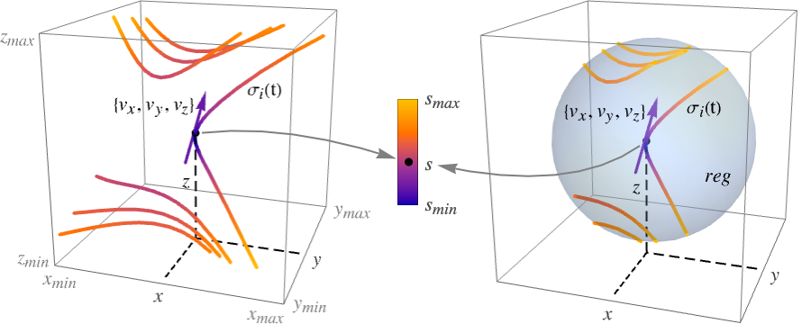
- StreamPlot3D plots streamlines
 defined by
  and
and  , where
  and
and  is an initial stream point. The streamline
  is the curve passing through point
  , and whose tangents correspond to the vector field
  at each point.
 - The streamlines are colored by default according to the magnitude
 of the vector field
  .
. - StreamPlot3D by default shows enough streamlines to achieve a roughly uniform density throughout the plot and shows no background scalar field.
- StreamPlot3D treats the variables x, y and z as local, effectively using Block.
- StreamPlot3D has attribute HoldAll and evaluates the vi etc. only after assigning specific numerical values to x, y and z. In some cases, it may be more efficient to use Evaluate to evaluate the vi etc. symbolically first.
- StreamPlot3D has the same options as Graphics3D, with the following additions and changes: [List of all options]
-
BoxRatios {1,1,1} ratio of height to width EvaluationMonitor None expression to evaluate at every function evaluation Method Automatic methods to use for the plot PerformanceGoal $PerformanceGoal aspects of performance to try to optimize PlotLegends None legends to include PlotRange {Full,Full,Full} range of x, y, z values to include PlotRangePadding Automatic how much to pad the range of values PlotTheme $PlotTheme overall theme for the plot RegionBoundaryStyle Automatic how to style plot region boundaries RegionFunction True& determine what region to include ScalingFunctions None how to scale individual coordinates StreamColorFunction Automatic how to color streamlines StreamColorFunctionScaling True whether to scale the argument to StreamColorFunction StreamMarkers Automatic shape to use for streams StreamPoints Automatic the number or placement of streamlines StreamScale None how to scale the sizes of streamlines StreamStyle Automatic how to draw streamlines WorkingPrecision MachinePrecision precision to use in internal computations - The arguments supplied to functions in RegionFunction and StreamColorFunction are x,y,z,vx,vy,vz,Norm[{vx,vy,vz}].
- Possible settings for StreamMarkers include:
-
"Arrow" lines with 2D arrowheads 
"Arrow3D" tubes with 3D arrowheads 
"Line" lines 
"Tube" tubes 
"Ribbon" flat ribbons 
"ArrowRibbon" ribbons with built-in arrowheads - With StreamScaleAutomatic and "arrow" stream markers, the streamlines are split into segments to make it easier to see the direction of the streamlines.
- Possible settings for StreamScale are:
-
Automatic automatically determine the streamline segments Full show the streamline as one piece Tiny,Small,Medium,Large named settings for how long the segments should be {len,npts,ratio} use explicit specification of streamline segmentation - The length len of streamline segments can be one of the following forms:
-
Automatic automatically determine the length None show the streamline as one piece Tiny,Small,Medium,Large use named segment lengths s use a length s that is a fraction of the graphic size - The number of points npts used to draw each segment can be Automatic or a specific number of points.
- The aspect ratio ratio specifies how wide the cross section of a streamline is relative to the streamline segment.
- Possible settings for ScalingFunctions include:
-
{sx,sy,sz} scale x, y and z axes - Common built-in scaling functions s include:
-
"Log" 
log scale with automatic tick labeling "Log10" 
base-10 log scale with powers of 10 for ticks "SignedLog" 
log-like scale that includes 0 and negative numbers "Reverse" 
reverse the coordinate direction "Infinite" 
infinite scale
List of all options
Examples
open all close allBasic Examples (4)
Plot streamlines through a vector field in 3D:
StreamPlot3D[{x, y, 1}, {x, -1, 1}, {y, -1, 1}, {z, -1, 1}]Use tubes to show the streamlines:
StreamPlot3D[{y^2, 1, x}, {x, -1, 1}, {y, -1, 1}, {z, -1, 1}, StreamMarkers -> "Tube"]Include a legend for the vector field magnitudes:
StreamPlot3D[{1, y, ArcTan[x]}, {x, -1, 1}, {y, -1, 1}, {z, -1, 1}, PlotLegends -> Automatic]Plot streamlines over an arbitrary region:
StreamPlot3D[{z, -x, y}, {x, y, z}∈Ball[]]Scope (12)
Sampling (3)
Specify the density of seed points for the streamlines:
StreamPlot3D[{x, y, 1}, {x, -1, 1}, {y, -1, 1}, {z, -1, 1}, StreamPoints -> Coarse]Specify specific seed points for the streamlines:
StreamPlot3D[{x, y, 1}, {x, -1, 1}, {y, -1, 1}, {z, -1, 1}, StreamPoints -> RandomReal[{-1, 1}, {30, 3}]]Plot streamlines over a specified region:
StreamPlot3D[{x, y, 1}, {x, -1, 1}, {y, -1, 1}, {z, -1, 1}, RegionFunction -> Function[{x, y, z}, x^2 + y^2 ≤ 1]]Presentation (9)
Streamlines are drawn as lines by default:
StreamPlot3D[{y, -x, y - x}, {x, -1, 1}, {y, -1, 1}, {z, -1, 1}]Use 3D tubes for the streamlines:
StreamPlot3D[{y, -x, y - x}, {x, -1, 1}, {y, -1, 1}, {z, -1, 1}, StreamMarkers -> "Tube"]StreamPlot3D[{y, -x, y - x}, {x, -1, 1}, {y, -1, 1}, {z, -1, 1}, StreamMarkers -> "Ribbon"]Use "arrow" versions of the stream markers to indicate the direction of flow along the streamlines:
StreamPlot3D[{z, -x, y + x}, {x, -1, 1}, {y, -1, 1}, {z, -1, 1}, StreamMarkers -> "Arrow"]StreamPlot3D[{z, -x, y + x}, {x, -1, 1}, {y, -1, 1}, {z, -1, 1}, StreamMarkers -> "Arrow3D"]Ribbons are turned into arrows by tapering the heads and notching the tails of the streamlines:
StreamPlot3D[{z, -x, y + x}, {x, -1, 1}, {y, -1, 1}, {z, -1, 1}, StreamMarkers -> "ArrowRibbon"]Use a single color for the streamlines:
StreamPlot3D[{y, -x, y - x}, {x, -1, 1}, {y, -1, 1}, {z, -1, 1}, StreamColorFunction -> None]Use a named color gradient for the streamlines:
StreamPlot3D[{y, -x, y - x}, {x, -1, 1}, {y, -1, 1}, {z, -1, 1}, StreamColorFunction -> "DarkRainbow"]Include a legend for the field magnitude:
StreamPlot3D[{y, -x, y - x}, {x, -1, 1}, {y, -1, 1}, {z, -1, 1}, PlotLegends -> Automatic]Use StreamScale to split streamlines into multiple shorter line segments:
StreamPlot3D[{x, y, 1}, {x, -1, 1}, {y, -1, 1}, {z, -1, 1}, StreamScale -> 0.1]StreamPlot3D[{x, y, 1}, {x, -1, 1}, {y, -1, 1}, {z, -1, 1}, StreamScale -> 0.2]Increase the number of points in each segment and increase the marker aspect ratio:
StreamPlot3D[{x, y, 1}, {x, -1, 1}, {y, -1, 1}, {z, -1, 1}, StreamMarkers -> "Arrow", StreamScale -> {Full, 20, 0.2}]StreamPlot3D[{x, y, 1}, {x, -1, 1}, {y, -1, 1}, {z, -1, 1}, PlotTheme -> "Marketing"]Use a log scale for the x axis:
StreamPlot3D[{x, y, z}, {x, 1, 100}, {y, 1, 100}, {z, 1, 100}, ScalingFunctions -> {"Log", None, None}]Reverse the y scale so it increases toward the bottom:
StreamPlot3D[{x, y, z}, {x, 1, 100}, {y, 1, 100}, {z, 1, 100}, ScalingFunctions -> {None, None, "Reverse"}]Options (70)
Axes (3)
By default, Axes are drawn:
StreamPlot3D[{y - z, z - x, x - y}, {x, -2, 2}, {y, -1, 1}, {z, -1, 1}]Use AxesFalse to turn off axes:
StreamPlot3D[{y - z, z - x, x - y}, {x, -2, 2}, {y, -1, 1}, {z, -1, 1}, Axes -> False]Turn each axis on individually:
{StreamPlot3D[{y - z, z - x, x - y}, {x, -2, 2}, {y, -1, 1}, {z, -1, 1}, Axes -> {True, False, False}], StreamPlot3D[{y - z, z - x, x - y}, {x, -2, 2}, {y, -1, 1}, {z, -1, 1}, Axes -> {False, True, False}], StreamPlot3D[{y - z, z - x, x - y}, {x, -2, 2}, {y, -1, 1}, {z, -1, 1}, Axes -> {False, False, True}]}AxesLabel (3)
No axes labels are drawn by default:
StreamPlot3D[{y - z, z - x, x - y}, {x, -2, 2}, {y, -1, 1}, {z, -1, 1}]StreamPlot3D[{y - z, z - x, x - y}, {x, -2, 2}, {y, -1, 1}, {z, -1, 1}, AxesLabel -> z]StreamPlot3D[{y - z, z - x, x - y}, {x, -2, 2}, {y, -1, 1}, {z, -1, 1}, AxesLabel -> {x, y, z}]AxesOrigin (2)
The position of the axes is determined automatically:
StreamPlot3D[{y - z, z - x, x - y}, {x, -2, 2}, {y, -1, 1}, {z, -1, 1}]Specify an explicit origin for the axes:
StreamPlot3D[{y - z, z - x, x - y}, {x, -2, 2}, {y, -1, 1}, {z, -1, 1}, AxesOrigin -> {2, -1, 1}]AxesStyle (4)
Change the style for the axes:
StreamPlot3D[{y - z, z - x, x - y}, {x, -2, 2}, {y, -1, 1}, {z, -1, 1}, AxesStyle -> StandardRed]Specify the style of each axis:
StreamPlot3D[{y - z, z - x, x - y}, {x, -2, 2}, {y, -1, 1}, {z, -1, 1}, AxesStyle -> {{Thick, StandardBrown}, {Thick, StandardBlue}, {Thick, StandardGreen}}]Use different styles for the ticks and the axes:
StreamPlot3D[{y - z, z - x, x - y}, {x, -2, 2}, {y, -1, 1}, {z, -1, 1}, AxesStyle -> StandardGreen, TicksStyle -> StandardGray]Use different styles for the labels and the axes:
StreamPlot3D[{y - z, z - x, x - y}, {x, -2, 2}, {y, -1, 1}, {z, -1, 1}, AxesStyle -> StandardGreen, LabelStyle -> StandardGray]BoxRatios (2)
By default, BoxRatios is set to Automatic:
StreamPlot3D[{y - z, z - x, x - y}, {x, -2, 2}, {y, -1, 1}, {z, -1, 1}]Make the box twice as long in the x direction:
StreamPlot3D[{y - z, z - x, x - y}, {x, -2, 2}, {y, -1, 1}, {z, -1, 1}, BoxRatios -> {2, 1, 1}]ImageSize (7)
Use named sizes, such as Tiny, Small, Medium and Large:
{StreamPlot3D[{y, -x, y - x}, {x, -1, 1}, {y, -1, 1}, {z, -1, 1}, ImageSize -> Tiny], StreamPlot3D[{y, -x, y - x}, {x, -1, 1}, {y, -1, 1}, {z, -1, 1}, ImageSize -> Small]}Specify the width of the plot:
{StreamPlot3D[{y, -x, y - x}, {x, -1, 1}, {y, -1, 1}, {z, -1, 1}, ImageSize -> 150], StreamPlot3D[{y, -x, y - x}, {x, -1, 1}, {y, -1, 1}, {z, -1, 1}, AspectRatio -> 1.5, ImageSize -> 150]}Specify the height of the plot:
{StreamPlot3D[{y, -x, y - x}, {x, -1, 1}, {y, -1, 1}, {z, -1, 1}, ImageSize -> {Automatic, 150}], StreamPlot3D[{y, -x, y - x}, {x, -1, 1}, {y, -1, 1}, {z, -1, 1}, AspectRatio -> 2, ImageSize -> {Automatic, 150}]}Allow the width and height to be up to a certain size:
{StreamPlot3D[{y, -x, y - x}, {x, -1, 1}, {y, -1, 1}, {z, -1, 1}, ImageSize -> UpTo[200]], StreamPlot3D[{y, -x, y - x}, {x, -1, 1}, {y, -1, 1}, {z, -1, 1}, AspectRatio -> 2, ImageSize -> UpTo[200]]}Specify the width and height for a graphic, padding with space if necessary:
StreamPlot3D[{y, -x, y - x}, {x, -1, 1}, {y, -1, 1}, {z, -1, 1}, ImageSize -> {200, 300}, Background -> StandardBlue]Setting AspectRatioFull will fill the available space:
StreamPlot3D[{y, -x, y - x}, {x, -1, 1}, {y, -1, 1}, {z, -1, 1}, AspectRatio -> Full, ImageSize -> {200, 300}, Background -> StandardBlue]Use maximum sizes for the width and height:
{StreamPlot3D[{y, -x, y - x}, {x, -1, 1}, {y, -1, 1}, {z, -1, 1}, ImageSize -> {UpTo[150], UpTo[100]}], StreamPlot3D[{y, -x, y - x}, {x, -1, 1}, {y, -1, 1}, {z, -1, 1}, AspectRatio -> 2, ImageSize -> {UpTo[150], UpTo[100]}]}Use ImageSizeFull to fill the available space in an object:
Framed[Pane[StreamPlot3D[{y, -x, y - x}, {x, -1, 1}, {y, -1, 1}, {z, -1, 1}, ImageSize -> Full, Background -> StandardBlue], {200, 200}]]Specify the image size as a fraction of the available space:
Framed[Pane[StreamPlot3D[{y, -x, y - x}, {x, -1, 1}, {y, -1, 1}, {z, -1, 1}, AspectRatio -> Full, ImageSize -> {Scaled[0.5], Scaled[0.5]}, Background -> StandardBlue], {200, 200}]]PlotLegends (3)
No legends are included by default:
StreamPlot3D[{y z, x z, x y}, {x, -1, 1}, {y, -1, 1}, {z, -1, 1}]Include a legend that indicates the vector field norm:
StreamPlot3D[{y z, x z, x y}, {x, -1, 1}, {y, -1, 1}, {z, -1, 1}, PlotLegends -> Automatic]Specify the location of the legend:
StreamPlot3D[{y z, x z, x y}, {x, -1, 1}, {y, -1, 1}, {z, -1, 1}, PlotLegends -> Placed[Automatic, Left]]PlotTheme (1)
RegionBoundaryStyle (4)
Show the region defined by a RegionFunction:
StreamPlot3D[{-4 x^2 y - 4 y^3 - x z, 4 x^3 + 4 x y^2 - y z, x^2 + y^2}, {x, -1, 1}, {y, -1, 1}, {z, -1, 1}, RegionFunction -> (#1^2 + #2^2 + #3^2 < 1&)]Use None to avoid showing the boundary:
StreamPlot3D[{-4 x^2 y - 4 y^3 - x z, 4 x^3 + 4 x y^2 - y z, x^2 + y^2}, {x, -1, 1}, {y, -1, 1}, {z, -1, 1}, RegionFunction -> (#1^2 + #2^2 + #3^2 < 1&), RegionBoundaryStyle -> None]Specify the color of the region boundary:
StreamPlot3D[{-4 x^2 y - 4 y^3 - x z, 4 x^3 + 4 x y^2 - y z, x^2 + y^2}, {x, -1, 1}, {y, -1, 1}, {z, -1, 1}, RegionFunction -> (#1^2 + #2^2 + #3^2 < 1&), RegionBoundaryStyle -> Orange]The boundaries of full rectangular regions are not shown:
StreamPlot3D[{-4 x^2 y - 4 y^3 - x z, 4 x^3 + 4 x y^2 - y z, x^2 + y^2}, {x, -1, 1}, {y, -1, 1}, {z, -1, 1}]RegionFunction (4)
StreamPlot3D[{-4 x^2 y - 4 y^3 - x z, 4 x^3 + 4 x y^2 - y z, x^2 + y^2}, {x, -1, 1}, {y, -1, 1}, {z, -1, 1}, RegionFunction -> (#1^2 + #2^2 + #3^2 < 1&)]Plot streams only where the field magnitude exceeds a given threshold:
StreamPlot3D[{-4 x^2 y - 4 y^3 - x z, 4 x^3 + 4 x y^2 - y z, x^2 + y^2}, {x, -1, 1}, {y, -1, 1}, {z, -1, 1}, RegionFunction -> (#7 > 2&)]Region functions depend, in general, on seven arguments:
StreamPlot3D[{x, y, 1}, {x, -2, 2}, {y, -2, 2}, {z, -2, 2}, RegionFunction -> Function[{x, y, z, vx, vy, vz, n}, vx vy > 0]]Use RegionBoundaryStyleNone to avoid showing the boundary:
StreamPlot3D[{-4 x^2 y - 4 y^3 - x z, 4 x^3 + 4 x y^2 - y z, x^2 + y^2}, {x, -1, 1}, {y, -1, 1}, {z, -1, 1}, RegionFunction -> (#1^2 + #2^2 + #3^2 < 1&), RegionBoundaryStyle -> None]ScalingFunctions (1)
Use a log scale for the x axis:
StreamPlot3D[{x, y, z}, {x, 1, 100}, {y, 1, 10}, {z, 1, 10}, ScalingFunctions -> {"Log", None, None}]Reverse the y scale so it increases toward the bottom:
StreamPlot3D[{x, y, z}, {x, 1, 100}, {y, 1, 100}, {z, 1, 100}, ScalingFunctions -> {None, None, "Reverse"}]StreamColorFunction (4)
Color the streams by their norm:
StreamPlot3D[{x, 2y, 3z}, {x, -1, 1}, {y, -1, 1}, {z, -1, 1}, StreamColorFunction -> Hue]Use any named color gradient from ColorData:
StreamPlot3D[{x, 2y, 3z}, {x, -1, 1}, {y, -1, 1}, {z, -1, 1}, StreamColorFunction -> "Rainbow"]Color the streamlines according to their x value:
StreamPlot3D[{x, 2y, 3z}, {x, -1, 1}, {y, -1, 1}, {z, -1, 1}, StreamColorFunction -> Function[{x, y, z, vx, vy, vz, n}, Hue[x]]]Use StreamColorFunctionScalingFalse to get unscaled values:
StreamPlot3D[{x, 2y, 3z}, {x, -1, 1}, {y, -1, 1}, {z, -1, 1}, StreamColorFunction -> "Rainbow", StreamColorFunctionScaling -> False]StreamColorFunctionScaling (2)
By default, scaled values are used:
StreamPlot3D[{y, -x, 10z}, {x, -1, 1}, {y, -1, 1}, {z, -1, 1}, StreamColorFunction -> "Pastel", PlotLegends -> Automatic]Use StreamColorFunctionScalingFalse to get unscaled values:
StreamPlot3D[{y, -x, 10z}, {x, -1, 1}, {y, -1, 1}, {z, -1, 1}, StreamColorFunction -> "BlueGreenYellow", PlotLegends -> Automatic, StreamColorFunctionScaling -> False]StreamMarkers (5)
StreamPlot3D[{-4 x^2 y - 4 y^3 - x z, 4 x^3 + 4 x y^2 - y z, x^2 + y^2}, {x, -1, 1}, {y, -1, 1}, {z, -1, 1}]Draw the streamlines as tubes:
StreamPlot3D[IconizedObject[«field»], IconizedObject[«vars»], StreamMarkers -> "Tube"]StreamPlot3D[IconizedObject[«field»], IconizedObject[«vars»], StreamMarkers -> "Ribbon"]"Arrow" stream markers automatically break the streamlines into shorter segments:
StreamPlot3D[IconizedObject[«field»], IconizedObject[«vars»], StreamMarkers -> "Arrow"]StreamPlot3D[IconizedObject[«field»], IconizedObject[«vars»], StreamMarkers -> "Arrow3D"]StreamPlot3D[IconizedObject[«field»], IconizedObject[«vars»], StreamMarkers -> "ArrowRibbon"]Make segmented markers continuous:
StreamPlot3D[{x, y, 1}, {x, -1, 1}, {y, -1, 1}, {z, -1, 1}, StreamMarkers -> "Arrow3D", StreamScale -> Full]Break continuous markers into segments:
StreamPlot3D[{x, y, 1}, {x, -1, 1}, {y, -1, 1}, {z, -1, 1}, StreamMarkers -> "Ribbon", StreamScale -> 0.1]StreamPoints (4)
Use automatically determined stream points to seed the curves:
StreamPlot3D[{y^2, 1, x}, {x, -1, 1}, {y, -1, 1}, {z, -1, 1}]Specify a maximum number of streamlines:
StreamPlot3D[{y^2, 1, x}, {x, -1, 1}, {y, -1, 1}, {z, -1, 1}, StreamPoints -> 25]Give specific seed points for the streams:
StreamPlot3D[{y^2, 1, x}, {x, -1, 1}, {y, -1, 1}, {z, -1, 1}, StreamPoints -> RandomReal[{-1, 1}, {20, 3}]]Use coarsely spaced streamlines:
StreamPlot3D[{y^2, 1, x}, {x, -1, 1}, {y, -1, 1}, {z, -1, 1}, StreamPoints -> Coarse]Use more finely spaced streamlines:
StreamPlot3D[{y^2, 1, x}, {x, -1, 1}, {y, -1, 1}, {z, -1, 1}, StreamPoints -> Fine]StreamScale (9)
Segmented markers have default lengths, numbers of points and aspect ratios:
StreamPlot3D[{1, y, ArcTan[x]}, {x, -1, 1}, {y, -1, 1}, {z, -1, 1}, StreamMarkers -> "Arrow"]Modify the lengths of the segments:
StreamPlot3D[{1, y, ArcTan[x]}, {x, -1, 1}, {y, -1, 1}, {z, -1, 1}, StreamMarkers -> "Arrow", StreamScale -> 0.2]Specify the number of sample points in each segment:
StreamPlot3D[{1, y, ArcTan[x]}, {x, -1, 1}, {y, -1, 1}, {z, -1, 1}, StreamMarkers -> "Arrow", StreamScale -> {0.2, 2}]Modify the aspect ratios for the stream markers:
StreamPlot3D[{1, y, ArcTan[x]}, {x, -1, 1}, {y, -1, 1}, {z, -1, 1}, StreamMarkers -> "Arrow", StreamScale -> {0.2, 2, 0.2}]Make segmented markers continuous:
StreamPlot3D[{1, y, ArcTan[x]}, {x, -1, 1}, {y, -1, 1}, {z, -1, 1}, StreamMarkers -> "Arrow", StreamScale -> Full]Break continuous markers into segments:
StreamPlot3D[{1, y, ArcTan[x]}, {x, -1, 1}, {y, -1, 1}, {z, -1, 1}, StreamMarkers -> "Ribbon", StreamScale -> 0.2]The aspect ratio controls the thickness of ribbons and tubes:
{StreamPlot3D[{1, y, ArcTan[x]}, {x, -1, 1}, {y, -1, 1}, {z, -1, 1}, StreamMarkers -> "Ribbon", StreamScale -> {Automatic, Automatic, 0.05}], StreamPlot3D[{1, y, ArcTan[x]}, {x, -1, 1}, {y, -1, 1}, {z, -1, 1}, StreamMarkers -> "Tube", StreamScale -> {Automatic, Automatic, 0.05}]}Increase the width of the ribbons and tubes:
{StreamPlot3D[{1, y, ArcTan[x]}, {x, -1, 1}, {y, -1, 1}, {z, -1, 1}, StreamMarkers -> "Ribbon", StreamScale -> {Automatic, Automatic, 0.1}], StreamPlot3D[{1, y, ArcTan[x]}, {x, -1, 1}, {y, -1, 1}, {z, -1, 1}, StreamMarkers -> "Tube", StreamScale -> {Automatic, Automatic, 0.1}]}The aspect ratio controls the sizes of arrowheads:
{StreamPlot3D[{1, y, ArcTan[x]}, {x, -1, 1}, {y, -1, 1}, {z, -1, 1}, StreamMarkers -> "Arrow", StreamScale -> {Automatic, Automatic, 0.15}], StreamPlot3D[{1, y, ArcTan[x]}, {x, -1, 1}, {y, -1, 1}, {z, -1, 1}, StreamMarkers -> "Arrow", StreamScale -> {Automatic, Automatic, 0.2}]}Control the number of points in each segment:
{StreamPlot3D[{-4 x^2 y - 4 y^3 - x z, 4 x^3 + 4 x y^2 - y z, x^2 + y^2}, {x, -1, 1}, {y, -1, 1}, {z, -1, 1}, StreamScale -> {0.5, 5}, ...], StreamPlot3D[{-4 x^2 y - 4 y^3 - x z, 4 x^3 + 4 x y^2 - y z, x^2 + y^2}, {x, -1, 1}, {y, -1, 1}, {z, -1, 1}, StreamScale -> {0.5, 20}, ...]}StreamStyle (3)
Change the appearance of the streamlines:
StreamPlot3D[{x, y, 1}, {x, -1, 1}, {y, -1, 1}, {z, -1, 1}, StreamStyle -> Thickness[0.02]]StreamColorFunction takes precedence over StreamStyle:
StreamPlot3D[{x, y, 1}, {x, -1, 1}, {y, -1, 1}, {z, -1, 1}, StreamStyle -> Directive[Red, Dashing[{0.1, 0.01}]]]Use StreamColorFunctionNone to specify a streamline color with StreamStyle:
StreamPlot3D[{x, y, 1}, {x, -1, 1}, {y, -1, 1}, {z, -1, 1}, StreamStyle -> Directive[StandardRed, Dashing[{0.1, 0.01}]], StreamColorFunction -> None]Ticks (6)
Ticks are placed automatically in each plot:
StreamPlot3D[{x, y, 1 / y}, {x, -2, 2}, {y, -2, 2}, {z, -2, 2}]Use TicksNone to not draw any tick marks:
StreamPlot3D[{x, y, 1 / y}, {x, -2, 2}, {y, -2, 2}, {z, -2, 2}, Ticks -> None]Place tick marks at specific positions:
StreamPlot3D[{x, y, 1 / y}, {x, -2, 2}, {y, -2, 2}, {z, -2, 2}, Ticks -> {{-1.5, 0, 1.5}, {-1.5, 0, 1.5}, {-1.5, 0, 1.5}}]Draw tick marks at the specified positions with the specified labels:
StreamPlot3D[{x, y, 1 / y}, {x, -2, 2}, {y, -2, 2}, {z, -2, 2}, Ticks -> {{{-1.5, -a}, {0, 0}, {1.5, a}}, {{-1.5, -a}, {0, 0}, {1.5, a}}, {{-1.5, -a}, {0, 0}, {1.5, a}}}]Specify tick marks with scaled lengths:
StreamPlot3D[{x, y, 1 / y}, {x, -2, 2}, {y, -2, 2}, {z, -2, 2}, Ticks -> {{{-1.5, -a, .1}, {0, 0, .1}, {1.5, a, .1}}, {{-1.5, -a, .05}, {0, 0, .05}, {1.5, a, .05}}, {{-1.5, -a, .15}, {0, 0, .15}, {1.5, a, .15}}}]Customize each tick with position, length, labeling and styling:
StreamPlot3D[{x, y, 1 / y}, {x, -2, 2}, {y, -2, 2}, {z, -2, 2}, Ticks -> {{{-1.5, -a, .1, Directive[Red, Dashed, Thick]}, {0, 0, .1, Directive[Red, Dashed]}, {1.5, a, .1, Directive[Red]}}, {{-1.5, -a, .05, Directive[StandardGray, Dashed, Thick]}, {0, 0, .05, Directive[StandardGray, Dashed]}, {1.5, a, .05, Directive[StandardGray]}}, {{-1.5, -a, .15, Directive[Darker@Green, Dashed, Thick]}, {0, 0, .15, Directive[Darker@Green, Dashed]}, {1.5, a, .15, Directive[Darker@Green]}}}]TicksStyle (3)
By default, the ticks and tick labels use the same styles as the axis:
StreamPlot3D[{x, y, 1 / y}, {x, -2, 2}, {y, -2, 2}, {z, -2, 2}, AxesStyle -> Directive[Bold, StandardRed]]Specify overall tick style, including the tick labels:
StreamPlot3D[{x, y, 1 / y}, {x, -2, 2}, {y, -2, 2}, {z, -2, 2}, TicksStyle -> Directive[Bold, StandardRed]]Specify tick style for each of the axes:
StreamPlot3D[{x, y, 1 / y}, {x, -2, 2}, {y, -2, 2}, {z, -2, 2}, TicksStyle -> {Directive[StandardGray, Bold], Directive[Bold, StandardRed], Directive[Bold, StandardBlue]}]Applications (10)
Basic Applications (1)
Consider a vector differential equation ![]() where
where ![]() is defined piecewise.
is defined piecewise.
Visualize solutions of ![]() using seed points for the streamlines that are inside the unit sphere:
using seed points for the streamlines that are inside the unit sphere:
StreamPlot3D[If[x^2 + y^2 + z^2 < 1, {x, y, z}, {1, 0, 0}], {x, -1.2, 1.2}, {y, -1.2, 1.2}, {z, -1.2, 1.2}, StreamPoints -> 0.5SpherePoints[50]]Fluid Flow (3)
Consider Stokes flow for a point force of the form ![]() , where
, where ![]() is a constant vector and
is a constant vector and ![]() is a Dirac delta function. For example, a force pointing down:
is a Dirac delta function. For example, a force pointing down:
F = {0, 0, -1};Define the fluid velocity vector ![]() , the pressure
, the pressure ![]() and the viscosity
and the viscosity ![]() :
:
vars = {x, y, z};
μ = 1;
u = (1/8π μ)Table[Sum[( (vars[[i]]vars[[j]]/(vars.vars)^3 / 2) + (IdentityMatrix[3][[i, j]]/Sqrt[vars.vars]))F[[j]], {j, 1, 3}], {i, 1, 3}];
p = (1/4π)Sum[(vars[[j]]F[[j]]/(vars.vars)^3 / 2), {j, 1, 3}];
Confirm that the equations for Stokes flow are satisfied so that ![]() and
and ![]() :
:
{Div[u, vars] == 0, Grad[p, vars] == μ Laplacian[u, vars]}//SimplifyPlot streamlines for the flow:
StreamPlot3D[u, {x, -3, 3}, {y, -3, 3}, {z, -3, 3}, StreamMarkers -> "Arrow3D", PlotLegends -> Automatic]Visualize Stokes flow around a unit sphere. Define the fluid velocity vector ![]() , the pressure
, the pressure ![]() , the viscosity
, the viscosity ![]() and the far-field fluid speed
and the far-field fluid speed ![]() :
:
vars = {x, y, z};
μ = 1;
U = 1;
u = {U, 0, 0} - (3/4)(x (U vars/(vars.vars)^3 / 2) + ({U, 0, 0}/Sqrt[vars.vars])) - (1/4)(({U, 0, 0}/(vars.vars)^3 / 2) - (3U x vars/(vars.vars)^5 / 2));
p = -(3μ x/2(vars.vars)^3 / 2);
Confirm that the equations for Stokes flow are satisfied so that ![]() and
and ![]() :
:
{Div[u, vars] == 0, Grad[p, vars] == μ Laplacian[u, vars]}//SimplifyPlot streamlines for the flow:
Show[StreamPlot3D[u, {x, -4, 4}, {y, -2, 2}, {z, -2, 2}, PlotLegends -> Automatic, StreamMarkers -> "Arrow", StreamPoints -> Flatten[Table[{-3, y, z}, {y, -1.75, 1.75, 0.5}, {z, -1.75, 1.75, 0.5}], 1]], Graphics3D[{Yellow, Sphere[]}], BoxRatios -> {2, 1, 1}]Plot the pressure for the flow:
DensityPlot3D[p, {x, -4, 4}, {y, -2, 2}, {z, -2, 2}, PlotLegends -> Automatic, RegionFunction -> Function[{x, y, z}, x^2 + y^2 + z^2 > 1], BoxRatios -> {2, 1, 1}]Specify the Navier–Stokes equations for a fluid through a pipe with a bulge:
velocities = {u[x, y, z], v[x, y, z], w[x, y, z]};
navierstokes = {
    Inactive[
       Div][(-μ Inactive[Grad][u[x, y, z], {x, y, z}]), {x, y,
       z}] + ρ  *
      velocities.Inactive[Grad][u[x, y, z], {x, y, z}] +
p^(1, 0, 0)[x, y, z],
    Inactive[
       Div][(-μ Inactive[Grad][v[x, y, z], {x, y, z}]), {x, y,
       z}] + ρ  *
      velocities.Inactive[Grad][v[x, y, z], {x, y, z}] +
p^(0, 1, 0)[x, y, z],
    Inactive[
       Div][(-μ Inactive[Grad][w[x, y, z], {x, y, z}]), {x, y,
       z}] + ρ  *
      velocities.Inactive[Grad][w[x, y, z], {x, y, z}] +
p^(0, 0, 1)[x, y, z],

u^(1, 0, 0)[x, y, z] + v^(0, 1, 0)[x, y, z] + w^(0, 0, 1)[x, y, z]} /. {μ -> 10 ^ -3, ρ -> 1};
Specify the geometry for the flow:
Ω = RegionUnion[Ball[], Cylinder[{{-2, 0, 0}, {2, 0, 0}}, 1 / 2]];
RegionPlot3D[Ω]
Specify the boundary conditions for flow from left to right:
inflowBC = DirichletCondition[{u[x, y, z] == 0.2, v[x, y, z] == 0, w[x, y, z] == 0}, x == -2];
outflowBC = DirichletCondition[p[x, y, z] == 0, x == 2];
wallBC = DirichletCondition[{u[x, y, z] == 0, v[x, y, z] == 0, w[x, y, z] == 0}, -2 < x < 2];
bcs = {inflowBC, outflowBC, wallBC};
Solve for the flow velocities and pressure:
{uVel, vVel, wVel, pressure} = NDSolveValue[{navierstokes == {0, 0, 0, 0}, bcs}, {u, v, w, p}, {x, y, z}∈Ω, Method -> {"FiniteElement", "InterpolationOrder" -> {u -> 2, v -> 2, w -> 2, p -> 1}, "MeshOptions" -> {"MaxCellMeasure" -> 0.01}}];Specify seed points for the streamlines:
sp = Prepend[#, 0]& /@ Flatten[Table[CirclePoints[r, 10], {r, {0.3, 0.5, 0.7, 0.9}}], 1];Plot the streamlines for the flow:
StreamPlot3D[{uVel[x, y, z], vVel[x, y, z], wVel[x, y, z]}, {x, -2, 2}, {y, -1, 1}, {z, -1, 1}, RegionFunction -> Function[{x, y, z}, {x, y, z}∈Ω], StreamPoints -> sp, BoxRatios -> {2, 1, 1}, Method -> {"IntegrationLimits" -> 100}, StreamMarkers -> "Arrow", StreamScale -> {0.05, Automatic, 0.07}, ImageSize -> Medium]Electrical Systems (1)
Visualize electric field lines for a dipole:
StreamPlot3D[({x, y, z - 1}/Norm[{x, y, z - 1}]^3) - ({x, y, z + 1}/Norm[{x, y, z + 1}]^3), {x, -3, 3}, {y, -3, 3}, {z, -3, 3}]The streamlines appear to have uniform color because of the extremely rapid change in the vector field norm near the point charges at ![]() . Bounding the magnitude of the vector field norm with a region function makes the colors visible:
. Bounding the magnitude of the vector field norm with a region function makes the colors visible:
StreamPlot3D[({x, y, z - 1}/Norm[{x, y, z - 1}]^3) - ({x, y, z + 1}/Norm[{x, y, z + 1}]^3), {x, -3, 3}, {y, -3, 3}, {z, -3, 3}, RegionFunction -> (#7 < 5&), RegionBoundaryStyle -> None, PlotLegends -> Automatic]Add spheres to indicate the positive (red) and negative (black) point charges:
Show[StreamPlot3D[({x, y, z - 1}/Norm[{x, y, z - 1}]^3) - ({x, y, z + 1}/Norm[{x, y, z + 1}]^3), {x, -3, 3}, {y, -3, 3}, {z, -3, 3}, RegionFunction -> (#7 < 5&), RegionBoundaryStyle -> None, PlotLegends -> Automatic], Graphics3D[{Red, Sphere[{0, 0, 1}, 0.2], Black, Sphere[{0, 0, -1}, 0.2]}]]Arrows can be used to provide more information, but the colors change because arrow markers are colored by the field magnitude at the tip of the arrow:
Show[StreamPlot3D[({x, y, z - 1}/Norm[{x, y, z - 1}]^3) - ({x, y, z + 1}/Norm[{x, y, z + 1}]^3), {x, -3, 3}, {y, -3, 3}, {z, -3, 3}, RegionFunction -> (#7 < 5&), RegionBoundaryStyle -> None, PlotLegends -> Automatic, StreamMarkers -> "Arrow3D"], Graphics3D[{StandardRed, Sphere[{0, 0, 1}, 0.2], StandardGray, Sphere[{0, 0, -1}, 0.2]}]]Use a custom StreamColorFunction to exert more control over the colors:
Show[StreamPlot3D[({x, y, z - 1}/Norm[{x, y, z - 1}]^3) - ({x, y, z + 1}/Norm[{x, y, z + 1}]^3), {x, -3, 3}, {y, -3, 3}, {z, -3, 3}, RegionFunction -> (0.01 < #7 < 5&), RegionBoundaryStyle -> None, StreamColorFunction -> (Blend[{GrayLevel[0], GrayLevel[1], RGBColor[1, 0, 0]}, #3]&), StreamMarkers -> "Arrow"], Graphics3D[{StandardRed, Sphere[{0, 0, 1}, 0.2], StandardGray, Sphere[{0, 0, -1}, 0.2]}]]Miscellaneous (5)
StreamPlot3D[{10(y - x), x(28 - z) - y, x y - (8/3) z}, {x, -30, 30}, {y, -30, 30}, {z, 0, 50}, StreamPoints -> {{1, 1, 1}}]Use ribbons or arrow ribbons to visualize the torsion of a twisted cubic:
StreamPlot3D[{1, 2x, 3x^2}, {x, -1, 1}, {y, -1, 1}, {z, -1, 1}, StreamMarkers -> "ArrowRibbon", StreamPoints -> {{0, 0, 0}}, ViewPoint -> {-1.3, 2.4, 2}]Visualize solutions of differential equations on manifolds:
StreamPlot3D[{-y, x, x^2 - y^2}, {x, -2, 2}, {y, -2, 2}, {z, -2, 2}, StreamPoints -> Table[{r, 0, 0}, {r, 0, 2, 0.2}]]Visualize streamlines for Poiseuille flow. The fluid speed is fastest along the central axis:
StreamPlot3D[{1 - y^2 - z^2, 0, 0}, {x, -2, 2}, {y, -1, 1}, {z, -1, 1}, BoxRatios -> {2, 1, 1}, PlotLegends -> Automatic, RegionFunction -> Function[{x, y, z}, y^2 + z^2 ≤ 1], StreamMarkers -> "Arrow", StreamPoints -> Flatten[Table[Prepend[#, 0]& /@ CirclePoints[r, 10], {r, 0.1, 1, 0.1}], 1]]Visualize solutions of Euler's equations for a rotating rigid body:
moments = {1, 2, 3};
StreamPlot3D[Evaluate[(| | | |
| --- | --- | --- |
| 0 | -x3 | x2 |
| x3 | 0 | -x1 |
| -x2 | x1 | 0 |).({x1, x2, x3}/moments)], {x1, -1, 1}, {x2, -1, 1}, {x3, -1, 1}, StreamPoints -> SpherePoints[40]]Properties & Relations (9)
Use VectorPlot3D to visualize a field with discrete arrows:
VectorPlot3D[{z, -x, y}, {x, -2, 2}, {y, -2, 2}, {z, -2, 2}]Use ListStreamPlot3D or ListVectorPlot3D to generate plots based on data:
data = Table[{z, -x, y}, {x, -2, 2}, {y, -2, 2}, {z, -2, 2}];{ListStreamPlot3D[data], ListVectorPlot3D[data]}Use StreamPlot to plot streamlines of 2D vector fields:
StreamPlot[{-1 - x ^ 2 + y, 1 + x - y ^ 2}, {x, -3, 3}, {y, -3, 3}]Use VectorPlot to plot with vectors instead of streamlines:
VectorPlot[{-1 - x ^ 2 + y, 1 + x - y ^ 2}, {x, -3, 3}, {y, -3, 3}]data = Table[{-1 - x ^ 2 + y, 1 + x - y ^ 2}, {x, -3, 3, 0.1}, {y, -3, 3, 0.1}];{ListStreamPlot[data], ListVectorPlot[data]}Use StreamDensityPlot to add a density plot of the scalar field:
StreamDensityPlot[{-1 - x ^ 2 + y, 1 + x - y ^ 2}, {x, -3, 3}, {y, -3, 3}]Use VectorDensityPlot to plot with arrows instead of streamlines:
VectorDensityPlot[{-1 - x ^ 2 + y, 1 + x - y ^ 2}, {x, -3, 3}, {y, -3, 3}]data = Table[{-1 - x ^ 2 + y, 1 + x - y ^ 2}, {x, -3, 3, 0.1}, {y, -3, 3, 0.1}];{ListStreamDensityPlot[data], ListVectorDensityPlot[data]}Use LineIntegralConvolutionPlot to plot the line integral convolution of a vector field:
LineIntegralConvolutionPlot[{-1 - x ^ 2 + y, 1 + x - y ^ 2}, {x, -3, 3}, {y, -3, 3}]Use VectorDisplacementPlot to visualize the deformation of a region associated with a displacement vector field:
VectorDisplacementPlot[{y, x - x^3}, {x, y}∈Disk[], VectorPoints -> Automatic]Use ListVectorDisplacementPlot to visualize the same deformation based on data:
data = Table[{{x, y} = RandomReal[{-1, 1}, {2}], {y, x - x ^ 3}}, {300}];ListVectorDisplacementPlot[data, Disk[], VectorPoints -> Automatic]Plot vectors along surfaces with SliceVectorPlot3D:
SliceVectorPlot3D[{x, y, z}, "CenterPlanes", {x, -1, 1}, {y, -1, 1}, {z, -1, 1}]data = Table[{x, y, z}, {x, -1, 1}, {y, -1, 1}, {z, -1, 1}];ListSliceVectorPlot3D[data, "CenterPlanes"]Use VectorDisplacementPlot3D to visualize the deformation of a 3D region associated with a displacement vector field:
VectorDisplacementPlot3D[{y, x, -z}, {x, 0, 1}, {y, 0, 1}, {z, 0, 1}, VectorPoints -> "Boundary"]Use ListVectorDisplacementPlot3D to visualize the same deformation based on data:
data = Table[{{x, y, z} = RandomReal[{0, 1}, {3}], {y, x, -z}}, {300}];ListVectorDisplacementPlot3D[data, Cuboid[], VectorPoints -> "Boundary"]Use ComplexVectorPlot or ComplexStreamPlot to visualize a complex function of a complex variable as a vector field or with streamlines:
{ComplexVectorPlot[Sin[3z], {z, 2}], ComplexStreamPlot[Sin[3z], {z, 2}]}Use GeoVectorPlot to plot vectors on a map:
GeoVectorPlot[GeoVector[GeoPosition[{{-54.79801473961214, -111.85053058521567},
    {-65.56940402358214, 162.89657500795147}, {-81.67990688759895, -93.36222177594851},
    {7.785750774919734, 95.44840765141487}, {-6.86571958448036, -40.946398330539864},
    { ... 904, "AngularDegrees"]},
   {0.9366099079317551, Quantity[357.70482317743733, "AngularDegrees"]},
   {0.8256817194791912, Quantity[242.07227508889662, "AngularDegrees"]},
   {0.2661401145642981, Quantity[152.90003252279325, "AngularDegrees"]}}]]
Use GeoStreamPlot to plot streamlines instead of vectors:
GeoStreamPlot[GeoVector[GeoPosition[{{-54.79801473961214, -111.85053058521567},
    {-65.56940402358214, 162.89657500795147}, {-81.67990688759895, -93.36222177594851},
    {7.785750774919734, 95.44840765141487}, {-6.86571958448036, -40.946398330539864},
    { ... 904, "AngularDegrees"]},
   {0.9366099079317551, Quantity[357.70482317743733, "AngularDegrees"]},
   {0.8256817194791912, Quantity[242.07227508889662, "AngularDegrees"]},
   {0.2661401145642981, Quantity[152.90003252279325, "AngularDegrees"]}}]]
Possible Issues (3)
Tube StreamMarkers can be distorted by the BoxRatios:
StreamPlot3D[{2, -10 z - x y, 10 y - x z}, {x, -2π, 2π}, {y, -1, 1}, {z, -1, 1}, StreamMarkers -> "Tube"]Carefully adjusting the BoxRatios can eliminate the tube distortion:
StreamPlot3D[{2, -10 z - x y, 10 y - x z}, {x, -2π, 2π}, {y, -1, 1}, {z, -1, 1}, StreamMarkers -> "Tube", BoxRatios -> {2π, 1, 1}]The colors of "Arrow" and "Arrow3D" stream markers are determined at the tip of the arrow, which can result in inconsistent colors for long arrows:
StreamPlot3D[{ArcTan[z], y, -x}, {x, -5, 5}, {y, -5, 5}, {z, -5, 5}]StreamPlot3D[{ArcTan[z], y, -x}, {x, -5, 5}, {y, -5, 5}, {z, -5, 5}, StreamMarkers -> "Arrow3D", StreamScale -> Full]Text
Wolfram Research (2021), StreamPlot3D, Wolfram Language function, https://reference.wolfram.com/language/ref/StreamPlot3D.html (updated 2022).
CMS
Wolfram Language. 2021. "StreamPlot3D." Wolfram Language & System Documentation Center. Wolfram Research. Last Modified 2022. https://reference.wolfram.com/language/ref/StreamPlot3D.html.
APA
Wolfram Language. (2021). StreamPlot3D. Wolfram Language & System Documentation Center. Retrieved from https://reference.wolfram.com/language/ref/StreamPlot3D.html