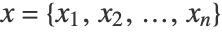
"LogisticRegression" (Machine Learning Method)
- Method for Classify.
- Models class probabilities with logistic functions of linear combinations of features.
Details & Suboptions
- "LogisticRegression" models the log probabilities of each class with a linear combination of numerical features
 ,
,  , where
 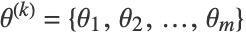 corresponds to the parameters for class k. The estimation of the parameter matrix
 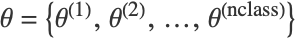 is done by minimizing the loss function
 ![sum_(i=1)^m-log(P_(theta)(class=y_i|x_i))+lambda_1 sum_(i=1)^nTemplateBox[{{theta, _, i}}, Abs]+(lambda_2)/2 sum_(i=1)^ntheta_i^2](Files/LogisticRegression.en/5.png "sum_(i=1)^m-log(P_(theta)(class=y_i|x_i))+lambda_1 sum_(i=1)^nTemplateBox[{{theta, _, i}}, Abs]+(lambda_2)/2 sum_(i=1)^ntheta_i^2") .
. - The following options can be given:
-
"L1Regularization" 0 value of  in the loss function
"L2Regularization" Automatic value of  in the loss function
"OptimizationMethod" Automatic what method to use - Possible settings for "OptimizationMethod" include:
-
"LBFGS" limited memory Broyden–Fletcher–Goldfarb–Shanno algorithm "StochasticGradientDescent" stochastic gradient method "Newton" Newton method
Examples
open all close allBasic Examples (2)
Train a classifier function on labeled examples:
c = Classify[{1, 2, 3, 4} -> {1, 1, 2, 2}, Method -> "LogisticRegression"]Obtain information about the classifier:
Information[c]c[1.3]Generate some normally distributed data:
sampledata[center_] := RandomVariate[MultinormalDistribution[center, IdentityMatrix[2]], 200];clusters = sampledata /@ {{1.5, 1}, {-1.5, 1}, {0, -3}};ListPlot[clusters, PlotStyle -> Darker@{Yellow, Blue, Green}]Train a classifier on this dataset:
c = Classify[<|Yellow -> clusters[[1]], Blue -> clusters[[2]], Green -> clusters[[3]]|>, Method -> "LogisticRegression"]Plot the training set and the probability distribution of each class as a function of the features:
Show[
	Plot3D[{
	c[{x, y}, "Probability" -> Yellow],
	c[{x, y}, "Probability" -> Blue],
	c[{x, y}, "Probability" -> Green]},
	{x, -4, 4}, {y, -5, 4},
	Exclusions -> None], ListPointPlot3D[Map[Append[#, 1]&, clusters, {2}], PlotStyle -> {Yellow, Blue, Green}]]
Options (6)
"L1Regularization" (2)
Train a classifier using the "L1Regularization" option:
c = Classify[<|1 -> {1, 23, 1.3, 4}, 2 -> {-4, -3.2, -4, -5}|>, Method -> {"LogisticRegression", "L1Regularization" -> 3}]Generate some data and visualize it:
colors = {RGBColor[1, 0, 0], RGBColor[0, 0, 1], RGBColor[0, 1, 0], RGBColor[1., 0.77, 0.]};
clusters = Table[RandomVariate[BinormalDistribution[
	RandomReal[{-3, 3}, 2],
	RandomReal[{0.5, 2}, 2],
	RandomReal[{0.2, 0.8}]], RandomInteger[{30, 40}]], {4}];
plot = ListPlot[clusters, PlotStyle -> Darker[colors, 0.1], ImageSize -> 200, PlotRange -> {{-5, 5}, {-5, 5}}, Frame -> True, AspectRatio -> 1, PlotLabel -> "data"]line = Range[-5, 5, 0.25];
points = Tuples[line, 2];makecolormap[probs_] := Transpose @ Partition[
Map[Blend[Keys[#], Values[#]]&, probs],
Length[line]];Train several classifiers using different values for "L1Regularization" and compare the results:
data = AssociationThread[colors, clusters];
Table[
ArrayPlot[
makecolormap @ Classify[data, points, "Probabilities", Method -> {"LogisticRegression", "L1Regularization" -> λ}],
PlotLabel -> ("L1Regularization" -> λ), DataReversed -> True, ImageSize -> 150],
{λ, {0, 3, 5, 10}}]~Multicolumn~2 ~Legended~plot"L2Regularization" (2)
Train a classifier using the "L2Regularization" option:
c = Classify[<|1 -> {1, 23, 1.3, 4}, 2 -> {-4, -3.2, -4, -5}|>, Method -> {"LogisticRegression", "L2Regularization" -> 3}]Generate some data and visualize it:
colors = {RGBColor[1, 0, 0], RGBColor[0, 0, 1], RGBColor[0, 1, 0], RGBColor[1., 0.77, 0.]};
clusters = Table[RandomVariate[BinormalDistribution[
RandomReal[{-4, 3}, 2],
RandomReal[{0.5, 2}, 2],
RandomReal[{0.2, 0.8}]], RandomInteger[{30, 40}]], {4}];
plot = ListPlot[clusters, PlotStyle -> Darker[colors, 0.1], ImageSize -> 200, PlotRange -> {{-5, 5}, {-5, 5}}, Frame -> True, AspectRatio -> 1, PlotLabel -> "data"]line = Range[-5, 5, 0.25];
points = Tuples[line, 2];Train several classifiers using different values for "L2Regularization" and compare the results:
makecolormap[probs_]  := Transpose @ Partition[
	Map[Blend[Keys[#], Values[#]]&, probs],
Length[line]];data = AssociationThread[colors, clusters];
Table[
ArrayPlot[
makecolormap @ Classify[data, points, "Probabilities", Method -> {"LogisticRegression", "L2Regularization" -> λ}],
PlotLabel -> ("L2Regularization" -> λ), DataReversed -> True, ImageSize -> 150],
{λ, {0, 3, 5, 10}}]~Multicolumn~2 ~Legended~plot"OptimizationMethod" (2)
Train a classifier using a specific "OptimizationMethod":
c = Classify[<|1 -> {1, 23, 1.3, 4}, 2 -> {-4, -3.2, -4, -5}|>, Method -> {"LogisticRegression", "OptimizationMethod" -> "StochasticGradientDescent"}]Train a classifier using the "Newton" method:
trainingset = {[image] -> 2, [image] -> 5, [image] -> 8, [image] -> 0, [image] -> 2, [image] -> 7, [image] -> 5, [image] -> 1, [image] -> 3, [image] -> 0, [image] -> 3, [image] -> 9, [image] -> 6, [image] -> 2, [image] -> 8, [image] -> 2, [image] -> 0, [image] -> 6, [image] -> 6, [image] -> 1, [image] -> 1, [image] -> 7, [image] -> 8, [image] -> 5, [image] -> 0, [image] -> 4, [image] -> 7, [image] -> 6, [image] -> 0, [image] -> 2, [image] -> 5, [image] -> 3, [image] -> 1, [image] -> 5, [image] -> 6, [image] -> 7, [image] -> 5, [image] -> 4, [image] -> 1, [image] -> 9, [image] -> 3, [image] -> 6, [image] -> 8, [image] -> 0, [image] -> 9, [image] -> 3, [image] -> 0, [image] -> 3, [image] -> 7, [image] -> 4, [image] -> 4, [image] -> 3, [image] -> 8, [image] -> 0, [image] -> 4, [image] -> 1, [image] -> 3, [image] -> 7, [image] -> 6, [image] -> 4, [image] -> 7, [image] -> 2, [image] -> 7, [image] -> 2, [image] -> 5, [image] -> 2, [image] -> 0, [image] -> 9, [image] -> 8, [image] -> 9, [image] -> 8, [image] -> 1, [image] -> 6, [image] -> 4, [image] -> 8, [image] -> 5, [image] -> 8, [image] -> 0, [image] -> 6, [image] -> 7, [image] -> 4, [image] -> 5, [image] -> 8, [image] -> 4, [image] -> 3, [image] -> 1, [image] -> 5, [image] -> 1, [image] -> 9, [image] -> 9, [image] -> 9, [image] -> 2, [image] -> 4, [image] -> 7, [image] -> 3, [image] -> 1, [image] -> 9, [image] -> 2, [image] -> 9, [image] -> 6};logistic = Classify[trainingset, Method -> {"LogisticRegression", "OptimizationMethod" -> "Newton"}]Train a classifier using the "StochasticGradientDescent" method:
logistic2 = Classify[trainingset, Method -> {"LogisticRegression", "OptimizationMethod" -> "StochasticGradientDescent"}]Compare the corresponding training times:
Information[logistic, "TrainingTime"]
Information[logistic2, "TrainingTime"]