有向グラフの階層的な描画
有向グラフの階層的な描画
LayeredGraphPlotは,グラフの頂点を「主」頂点を最上層とする階層的な一連の「層」で描こうとする.
| LayeredGraphPlot[{vi1->vj1,vi2->vj2,…}] | |
頂点 vik が頂点 vjk と接続しているグラフの階層的なプロットを生成する | |
| LayeredGraphPlot[{{vi1->vj1,lbl1},…}] | |
ラベル lblk をグラフ中の辺と関連付ける | |
| LayeredGraphPlot[g,pos] | グラフ中の主頂点を位置 pos に置く |
| LayeredGraphPlot[m] | 隣接行列 m で表されるグラフの階層的なプロットを生成する |
LayeredGraphPlotは,辺の方向が主に下向きになるようにグラフを描画する. LayeredGraphPlotの第2引数は根の位置を指定する.この引数に可能な値はRight,Left,Top,Bottomである.
LayeredGraphPlot[{4 -> 3, 5 -> 3, 5 -> 4, 6 -> 1, 6 -> 2, 6 -> 4, 6 -> 5, 6 -> 3}, VertexLabels -> Automatic]LayeredGraphPlot[{4 -> 3, 5 -> 3, 5 -> 4, 6 -> 1, 6 -> 2, 6 -> 4, 6 -> 5, 6 -> 3}, Left, VertexLabels -> Automatic]浮動小数点の相違のため,LayeredGraphPlotはプラットフォームによって異なる出力を生成することがある.
オプション名
|
デフォルト値
| |
| DataRange | Automatic | 生成する頂点座標の範囲 |
| DirectedEdges | True | 辺を有向の矢印として示すかどうか |
| EdgeLabels | Automatic | 辺に与えられたラベルを含めるかどうか |
| EdgeShapeFunction | Automatic | 辺の明示的なグラフィックスを与える関数 |
| MultiedgeStyle | Automatic | 頂点間の多重辺をどのように描くか |
| "PackingLayout" | Automatic | 要素のパッキングに使用するメソッド |
| PlotRangePadding | Automatic | プロット周囲にどの程度の充填を行うか |
| PlotStyle | Automatic | オブジェクトを描画するスタイル |
| SelfLoopStyle | Automatic | 頂点をそれ自身と結ぶ辺をどのように描くか |
| VertexCoordinates | Automatic | 明示的な頂点座標の規則 |
| VertexLabels | Automatic | 頂点名をラベルとして示すかどうか |
| VertexShapeFunction | Automatic | 頂点の明示的なグラフィックスを与える関数 |
LayeredGraphPlotのオプション
DirectedEdges
LayeredGraphPlot[{4 -> 3, 5 -> 2, 5 -> 3, 5 -> 4, 6 -> 1, 6 -> 2, 6 -> 4}, DirectedEdges -> False, VertexLabels -> Automatic]EdgeLabels
オプションEdgeLabelsは,辺に与えられたラベルを表示するかどうか,またどのように表示するかを指定する.このオプションが取り得る値はAll,NoneまたはAutomaticである.このオプションのデフォルト値はAutomaticで,与えられた辺のラベルをグラフに表示する.
LayeredGraphPlot[{1 -> 5, 1 -> 6, 2 -> 4, 2 -> 6, 3 -> 4, 3 -> 5, {3 -> 6, "edge 3->6"}, 4 -> 6, 5 -> 6}, VertexLabels -> Automatic]Tooltip[vi->vj,lab]を使って辺のツールチップを指定する.カーソルを頂点3と頂点6の間の辺の上,または頂点3と5の間の辺の上に置くとツールチップが見られる:
LayeredGraphPlot[{1 -> 5, 1 -> 6, 2 -> 4, 2 -> 6, 3 -> 4, {3 -> 5, Tooltip[ "edge 3->5", "3->5"]}, Tooltip[3 -> 6, "3->6"], 4 -> 6, 5 -> 6}, VertexLabels -> Automatic]EdgeShapeFunction
オプションEdgeShapeFunctionは,グラフの辺の視覚的表現を指定する.このオプションに可能な値はAutomatic,None,あるいはグラフィックスプリミティブとグラフィックス指示子との適切な組合せを与える関数である.デフォルト設定のAutomaticでは,各辺が暗赤色の線で描画される.EdgeShapeFunction->Noneでは,辺は描画されない.
LayeredGraphPlot[Table[1, {10}, {10}], EdgeShapeFunction -> None, VertexLabels -> Automatic]EdgeShapeFunction->g のとき,各辺は関数 g で与えられるグラフィックスプリミティブとグラフィックス指示子で描画される.この関数は g[{ri,…,rj},{vi,vj},lblij,…]という形式で3つ以上の引数を取ることができ,ri と rj は辺の始点と終点の座標,vi と vj は最初の頂点と最後の頂点,lblij は辺に指定された任意のラベルあるいはNoneである.EdgeShapeFunction->g の明示的な設定値はEdgeLabelsとDirectedEdgesの設定値に優先する.
LayeredGraphPlot[{1 -> 2, 2 -> 3, 3 -> 4, 4 -> 5, 5 -> 6, 6 -> 7, 7 -> 1, 11 -> 12, 12 -> 13, 13 -> 14, 14 -> 15, 15 -> 16, 16 -> 17, 17 -> 11, 1 -> 11, 2 -> 12, 3 -> 13, 4 -> 14, 5 -> 15, 6 -> 16, 7 -> 17}, EdgeShapeFunction -> ({GrayLevel[0.5], Arrow[#1, 0.3]}&)]LayeredGraphPlot[{1 -> 2, 2 -> 3, 3 -> 4, 5 -> 1, 5 -> 2, 5 -> 3, 5 -> 4, 1 -> 4, 3 -> 5, 3 -> 3}, EdgeShapeFunction -> ({If[First[#2] === Last[#2], Red, StandardGreen], Arrow[#1, .1]}&)]MultiedgeStyle
オプションMultiedgeStyleは,2つの頂点間の多重辺を描くかどうかを指定する.MultiedgeStyleが取り得る値はAutomatic(デフォルト),True,False,正の実数である.デフォルト設定のMultiedgeStyle->Automaticでは,規則のリストで指定されたグラフに対しては多重辺が表示されるが,隣接行列により指定された場合は表示されない.MultiedgeStyle->δ では,多重辺はスケールされた距離 δ にまで広げられる.
LayeredGraphPlot[{1 -> 2, 2 -> 1, 1 -> 2, 1 -> 2, 2 -> 3, 3 -> 5, 4 -> 5, 5 -> 6, 5 -> 1}, VertexLabels -> Automatic]LayeredGraphPlot[(| | | | | | |
| :- | :- | :- | :- | :- | :- |
| 0 | 3 | 0 | 0 | 0 | 0 |
| 1 | 0 | 1 | 0 | 0 | 0 |
| 0 | 0 | 0 | 0 | 1 | 0 |
| 0 | 0 | 0 | 0 | 1 | 0 |
| 1 | 0 | 0 | 0 | 0 | 1 |
| 0 | 0 | 0 | 0 | 0 | 0 |), VertexLabels -> Automatic]LayeredGraphPlot[{1 -> 2, 2 -> 1, 1 -> 2, 1 -> 2, 2 -> 3, 3 -> 5, 4 -> 5, 5 -> 6, 5 -> 1}, MultiedgeStyle -> 0.25, VertexLabels -> Automatic]PackingLayout
オプション"PackingLayout"は非連結要素をパッキングするためのメソッドを指定する.このオプションに可能な値はAutomatic(デフォルト),"ClosestPacking","ClosestPackingCenter","Layered","LayeredLeft","LayeredTop","NestedGrid"である."PackingLayout"->"ClosestPacking"では,要素は左上からポリオミノ法[6]を使って可能な限り近付くようパックされる."PackingLayout"->"ClosestPackingCenter"では,要素は中央からパックされる."PackingLayout"->"Layered"では,要素は左上から層状にパックされる."PackingLayout"->"LayeredLeft"あるいは"PackingLayout"->"LayeredTop"では,要素はそれぞれ上・左から層状にパックされる."PackingLayout"->"NestedGrid"では,要素はネストされた格子に配列される.通常効率的なデフォルト設定は"PackingLayout"->"Layered"であり,パッキングは最大の境界ボックス部分の要素から始まる.
LayeredGraphPlot[Table[i -> Mod[i ^ 3, 221], {i, 0, 221}], DirectedEdges -> False]LayeredGraphPlot[Table[i -> Mod[i ^ 3, 221], {i, 0, 221}], GraphLayout -> {"PackingLayout" -> "ClosestPackingCenter"}, DirectedEdges -> False]PlotRangePadding
PlotStyle
LayeredGraphPlot[{1 -> 2, 2 -> 3, 3 -> 4, 4 -> 1, 6 -> 5, 7 -> 5, 5 -> 4, 9 -> 8, 10 -> 8, 8 -> 3, 12 -> 11, 13 -> 11, 11 -> 1, 15 -> 14, 16 -> 14, 14 -> 2}, VertexLabels -> Automatic, PlotStyle -> {Red, Arrowheads[{{0.1, 0.8}}], Thickness[0.02]}]SelfLoopStyle
オプションSelfLoopStyleは,自分自身とリンクしている頂点のループを描くかどうかを指定する.このオプションに可能な値はAutomatic(デフォルト)True,False,正の実数である.SelfLoopStyle->Automaticでは,グラフが規則のリストで指定されている場合に自己ループが表示され,隣接行列で指定されている場合は表示されない.SelfLoopStyle->δ では,自己ループは直径 δ(辺の平均の長さに対して)で描画される.
LayeredGraphPlot[{3 -> 2, 4 -> 1, 4 -> 3, 5 -> 1, 5 -> 2, 6 -> 1, 6 -> 2, 6 -> 3, 6 -> 4, 6 -> 5, 1 -> 1, 1 -> 1}, VertexLabels -> Automatic]LayeredGraphPlot[(| | | | | | |
| :- | :- | :- | :- | :- | :- |
| 0 | 1 | 0 | 0 | 0 | 0 |
| 0 | 0 | 0 | 0 | 0 | 0 |
| 1 | 0 | 0 | 1 | 0 | 0 |
| 0 | 0 | 0 | 2 | 0 | 0 |
| 0 | 1 | 0 | 1 | 0 | 0 |
| 1 | 1 | 1 | 1 | 1 | 0 |), VertexLabels -> Automatic]LayeredGraphPlot[{3 -> 2, 4 -> 1, 4 -> 3, 5 -> 1, 5 -> 2, 6 -> 1, 6 -> 2, 6 -> 3, 6 -> 4, 6 -> 5, 1 -> 1, 1 -> 1}, VertexLabels -> Automatic, SelfLoopStyle -> 0.3]VertexCoordinates
LayeredGraphPlot[{1 -> 3, 1 -> 4, 2 -> 4, 2 -> 5, 3 -> 5, 6 -> 7, 7 -> 8, 8 -> 9, 9 -> 10, 6 -> 10, 1 -> 6, 2 -> 7, 3 -> 8, 4 -> 9, 5 -> 10}, VertexCoordinates -> {{0.309017, 0.951057}, {-0.809017, -0.587785}, {0.309017, -0.951057}, {-0.809017, 0.587785}, {1., 0}, {0.618034, 1.90211}, {-1.61803, 1.17557}, {-1.61803, -1.17557}, {0.618034, -1.90211}, {2., 0}}]LayeredGraphPlot[{1 -> 3, 1 -> 4, 2 -> 4, 2 -> 5, 3 -> 5, 6 -> 7, 7 -> 8, 8 -> 9, 9 -> 10, 6 -> 10, 1 -> 6, 2 -> 7, 3 -> 8, 4 -> 9, 5 -> 10}]VertexLabels
オプションVertexLabelsは頂点名をラベルとして表示するかどうかを指定する.このオプションに可能な値はAll,None,Automatic(デフォルト),Tooltipである.VertexLabels->Allではラベルが表示される.隣接行列で指定されたグラフでは,頂点ラベルは連続した整数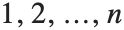 (n は行列の大きさ)を取る.規則のリストで指定されたグラフでは,ラベルは規則で使われた式である.VertexLabels->Noneでは各頂点は点として表示される.頂点 vk に対する別のツールチップを指定する場合は,規則のリストの任意の場所でTooltip[vk,vlbl]を使うとよい.
 LayeredGraphPlot[(| | | | | |
| :- | :- | :- | :- | :- |
| 0 | 1 | 0 | 0 | 0 |
| 0 | 0 | 0 | 0 | 0 |
| 1 | 1 | 0 | 0 | 0 |
| 0 | 1 | 0 | 0 | 0 |
| 0 | 1 | 0 | 0 | 0 |), VertexLabels -> Automatic]LayeredGraphPlot[{"A" -> "B", "A" -> "a", "B" -> "C", "C" -> "A"}, VertexLabels -> Automatic]LayeredGraphPlot[{"A" -> "B", "A" -> "a", "B" -> "C", "C" -> "A"}, VertexLabels -> Placed[Automatic, Tooltip]]VertexShapeFunction
オプションVertexShapeFunctionはグラフの辺の視覚的表現を指定する.このオプションに可能な値はAutomatic,None,あるいはグラフィックスプリミティブと指示子の適切な組合せを与える関数である.デフォルト設定のAutomaticでは,頂点は点として表示される.
g = {5 -> 3, 5 -> 4, 6 -> 2, 6 -> 4, 7 -> 1, 7 -> 4, 7 -> 5, 7 -> 6};LayeredGraphPlot[g]LayeredGraphPlot[g, VertexShapeFunction -> None]VertexShapeFunction->g では,各頂点が g[ri,vi,…]で与えられるグラフィックスプリミティブで描画される.ri は頂点の座標で,vi は頂点のラベルである.VertexShapeFunction->g の明示的な設定値はVertexLabelsの設定値に優先する.
LayeredGraphPlot[{1 -> 2, 2 -> 3, 3 -> 4, 4 -> 5, 5 -> 6, 6 -> 7, 7 -> 8, 8 -> 1, 1 -> 9, 2 -> 9, 3 -> 10, 4 -> 10, 6 -> 11, 5 -> 11, 7 -> 12, 8 -> 12}, Left, VertexShapeFunction -> ({EdgeForm[Black], Yellow, Disk[#1, 0.2], Black, Text[#2, #1]}&)]フローチャート
LayeredGraphPlotは,ビジネス,経済,技術的なプレゼンテーション等のためのフローチャートの可視化に役立つ.
LayeredGraphPlot[{"total" -> "TotalDispatch", "TotalList" -> "CheckThreading", "TotalList" -> "TotalDispatch", "TotalSparse" -> "TotalDispatch", "TotalSparse" -> "TotalDispatch", "TotalDispatch" -> "TotalDispatch", "TotalDispatch" -> "TotalList", "TotalDispatch" -> "TotalPacked", "TotalDispatch" -> "TotalSparse"}, VertexLabels -> Automatic]LayeredGraphPlot[{"ratiotest" -> "ratiolimit", "getdata" -> "dir_inf _bad", "getdata" -> "evalderiv", "NSPpreliminaries" -> "getdata", "findsp" -> "termlimit", "findsp" -> "ratiotest", "findsp" -> "nSumW", "findsp" -> "nSumEM", "findsp" -> "nProductEM", "findsp" -> "nProductW", "nSumW" -> "nSumFinite", "nSumW" -> "nSumWtail", "nSumEM" -> "evalterm", "nSumEM" -> "nSumFinite", "nSumEM" -> "evalderiv", "nProductEM" -> "nPFinite", "nProductW" -> "nPFinite", "nProductW" -> "nPWtail", "oNSum" -> "CleanOptionList", "oNSum" -> "multidim", "oNSum" -> "NSPpreliminaries", "oNSum" -> "findsp", "nSumFinite" -> "evalterm", "nSumWtail" -> "evalterm", "nSumWtail" -> "epsalg", "oNProduct" -> "CleanOptionList", "oNProduct" -> "multidim", "oNProduct" -> "NSPpreliminaries", "oNProduct" -> "findsp", "nPFinite" -> "evalterm", "nPWtail" -> "evalterm", "nPWtail" -> "epsalg", "oSequenceLimit" -> "epsalg"}, Left, VertexLabels -> Automatic, AspectRatio -> 1, PlotRangePadding -> 0.02]食物連鎖
食物連鎖はLayeredGraphPlotを使って可視化することができる.
LayeredGraphPlot[{"John" -> "plants",
  "lion" -> "John",   "tiger" -> "John", "tiger" -> "deer", "lion" -> "deer", "deer" -> "plants",
  "mosquito" -> "lion", "frog" -> "mosquito", "mosquito" -> "tiger", "John" -> "cow", "cow" -> "plants", "mosquito" -> "deer", "mosquito" -> "John", "snake" -> "frog", "vulture" -> "snake"}, Left,
VertexLabels -> Automatic]LayeredGraphPlot[ {"Raccoon" -> "Bird", "Raccoon" -> "Insect", "Wildcat" -> "Bird", "Wildcat" -> "Rodent", "Fox" -> "Bird", "Fox" -> "Garter snake", "Fox" -> "Salamander", "Fox" -> "Rabbit", "Fox" -> "Rodent", "Wolf" -> "Rabbit", "Wolf" -> "Rodent", "Wolf" -> "Skunk", "Wolf" -> "Deer", "Bear" -> "Deer", "Bear" -> "Rodent", "Bear" -> "Plant", "Bird" -> "Plant", "Garter snake" -> "Insect", "Garter snake" -> "Toad", "Salamander" -> "Insect", "Rabbit" -> "Plant", "Skunk" -> "Rodent", "Skunk" -> "Insect", "Deer" -> "Plant", "Toad" -> "Insect", "Insect" -> "Plant"}, VertexLabels -> Automatic, PlotRangePadding -> Automatic]Unixの歴史
LayeredGraphPlotは歴史的事象を可視化するのにも適している.
LayeredGraphPlot[{"5th Edition" -> "6th Edition", "5th Edition" -> "PWB 1.0",
  "6th Edition" -> "1 BSD", "6th Edition" -> "Interdata",
  "6th Edition" -> "LSX", "6th Edition" -> "Mini Unix",
  "6th Edition" -> "Wollongong", "PWB 1.0" -> "PWB 1.2",
  "PWB 1.0" -> "USG 1.0", "1 BSD" -> "2 BSD", "Interdata" -> "PWB 2.0",
  "Interdata" -> "Unix/TS 3.0", "Interdata" -> "7th Edition",
  "PWB 1.2" -> "PWB 2.0", "USG 1.0" -> "USG 2.0", "USG 1.0" -> "CB Unix 1",
  "7th Edition" -> "2 BSD", "7th Edition" -> "32V", "7th Edition" -> "Xenix",
  "7th Edition" -> "Ultrix-11", "7th Edition" -> "UniPlus+",
  "7th Edition" -> "V7M", "PWB 2.0" -> "Unix/TS 3.0", "USG 2.0" -> "USG 3.0",
  "CB Unix 1" -> "CB Unix 2", "32V" -> "3 BSD",
  "Unix/TS 1.0" -> "Unix/TS 3.0", "USG 3.0" -> "Unix/TS 3.0",
  "CB Unix 2" -> "CB Unix 3", "3 BSD" -> "4 BSD", "V7M" -> "Ultrix-11",
  "Unix/TS 3.0" -> "TS 4.0", "CB Unix 3" -> "Unix/TS++",
  "CB Unix 3" -> "PDP-11 Sys V", "4 BSD" -> "4.1 BSD",
  "Unix/TS++" -> "TS 4.0", "4.1 BSD" -> "8th Edition", "4.1 BSD" -> "4.2 BSD",
   "4.1 BSD" -> "2.8 BSD", "2 BSD" -> "2.8 BSD", "TS 4.0" -> "System V.0",
  "4.2 BSD" -> "4.3 BSD", "4.2 BSD" -> "Ultrix-32", "2.8 BSD" -> "2.9 BSD",
  "2.8 BSD" -> "Ultrix-11", "System V.0" -> "System V.2",
  "8th Edition" -> "9th Edition", "System V.2" -> "System V.3"}, VertexLabels -> Automatic, AspectRatio -> 0.7, PlotRangePadding -> Automatic]