Surgical fixation plate
The purpose of this notebook is to illustrate the usage of the OpenCascadeLink to create a surgical fixation plate based on a parametric design.
A surgical fixation plate is a medical device used to stabilize and support broken bones during the healing process. Titanium fixation plates, particularly those designed for the forearm, are favored for their strength, biocompatibility, and resistance to corrosion. These plates are surgically attached to the fractured bones using screws, ensuring proper alignment and promoting effective recovery. The usage of a parametric design allows for optimization procedures and easy personalization of the devices based on the patients needs.
The fixation plate design is based on an analytical description that leads to a parametric geometry function of the fixation plate's side length and the width. The creation procedure in OpenCascade starts with the description of the planar face which is then extruded to form the 3D object.

Surgical fixation plate (in brown) placed over the Radius in the forearm.
Needs["OpenCascadeLink`"]
Needs["NDSolve`FEM`"]
Geometry
The fixation plate is divided into a central section and two fixation sections at the sides. Both the fixation sections and the central section have three holes each.
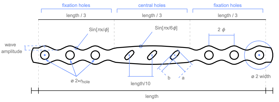
Two dimensional technical diagram of the planar surgical fixation plate with sizes expressed as a function of the desired length and width. The fixation plate is divided into three sections, each with a length of length/3.
To create the 3D geometry a 2D draft will be made that then can be extruded to 3D. To make this 2D draft, all edges will be parameterized and connected to form a planar 2D face. From that face the holes can be removed and in the last step the perforated face will be extruded to 3D.
The first step is to create the top edge of the 2D plate. This long edge can be split in three regions represented by a sine function scaled to fit the desired numbers of holes in each semi-period. The geometric properties are expressed in centimeters.
length = 16;
thickness = 0.3;
width = 1;
waveAmplitude = 0.15;numberFixationHoles = 3;
radiusFixationHoles = 0.3;A sine function is used to house the holes of the fixation plate within each positive wave cycle of the period. The period is determined by dividing the available length by twice the number of fixation holes.
ϕ = (length/3)(1/numberFixationHoles * 2)fixationEdge[x_] := Sin[(π x/ϕ)]centralEdge[x_] := fixationEdge[(x/6)]edge[x_] := (width/2) + waveAmplitude * Which[
x <= (length/3), fixationEdge[x],
(length/3) < x <= (length/2), -centralEdge[x]]edgePlot = Plot[edge[x + length / 2], {x, -length / 2, 0}, AspectRatio -> Automatic, ImageSize -> Large, Ticks -> {True, False}]The next step is to convert this plot of the edge into a spline. For that the edge is discretized and downsampled and converted to a BSplineCurve.
discretedEdge = DiscretizeGraphics[edgePlot]topEdgeCoords = MeshCoordinates[discretedEdge][[1 ;; -1 ;; 15]];topEdgeCoords[[-1, 1]] = 0.;Show[discretedEdge, Graphics[{Red, Point[topEdgeCoords]}]]topEdgeSpline = BSplineCurve[topEdgeCoords];
Graphics[topEdgeSpline]The next step is to create left edge of the geometry, which can be represented by a circular sector. The challenge is to find the exact size of the sector. To help in the process it is convenient to visualize a half circle and the top edge and an extension of the top edge that intersects with the half circle.
leftCircleCenter = {-length / 2 + width / 2, 0}circleSegement = Circle[leftCircleCenter, width, {π / 2, π}]extensionLine = Line[{topEdgeCoords[[1]], {leftCircleCenter[[1]] - width, topEdgeCoords[[1, 2]]}}]Graphics[{topEdgeSpline, {Red, extensionLine}, circleSegement}]Once the intersection of the extension line and the half circle is computed the left edge sector can be established.
intersectionPoint = RegionIntersection[extensionLine, circleSegement]leftIntersectionCoord = intersectionPoint[[1, 1]]leftIntersectAngle = NSolveValues[leftIntersectionCoord[[1]] == leftCircleCenter[[1]] + width * Cos[θ], θ, MaxRoots -> 1][[1]]leftLine = Line[{leftIntersectionCoord, topEdgeCoords[[1]]}];
leftEdge = Circle[leftCircleCenter, width, {2π - leftIntersectAngle, π}];
Graphics[{topEdgeSpline, {Red, leftLine}, leftEdge}]rt1 = ReflectionTransform[{1, 0}, {0, 0}];tr1 = TransformedRegion[topEdgeSpline, rt1];
tr2 = TransformedRegion[leftLine, rt1];
tr3 = TransformedRegion[leftEdge, rt1];
tr3 = tr3 /. Circle[c_List, r_, s_] :> Circle[c, r, {0, s[[1]]}];
Graphics[{topEdgeSpline, leftLine, leftEdge, {Blue, tr1}, {Red, tr2}, {Magenta, tr3}}]e1 = OpenCascadeShape[leftEdge];
e2 = OpenCascadeShape[leftLine];
e3 = OpenCascadeShape[topEdgeSpline];
e4 = OpenCascadeShape[tr1];
e5 = OpenCascadeShape[tr2];
e6 = OpenCascadeShape[tr3];w1 = OpenCascadeShapeWire[{e1, e2, e3, e4, e5, e6}]Next, the entire top half will be reflected to the bottom.
rt2 = ReflectionTransform[{0, -1}, {0, 0}];gt1 = GeometricTransformation[topEdgeSpline, rt2];
gt2 = GeometricTransformation[leftLine, rt2];
gt3 = GeometricTransformation[leftEdge, rt2];
Graphics[{topEdgeSpline, leftLine, leftEdge, {Blue, gt1}, {Red, gt2}, {Magenta, gt3}}]The actual transformation will operate on the entire top edge.
w2 = OpenCascadeShapeTransformation[w1, rt2]face = OpenCascadeShapeFace[{w1, w2}]bmesh = OpenCascadeShapeSurfaceMeshToBoundaryMesh[face];
bmesh["Wireframe"]The next step is to introduce the holes in the fixation plate. There are three group of holes: two groups of fixation holes and the central holes. The fixation holes are described by circles aligned with the sine spatial period ![]() , while the central holes are represented by an hyperelliptic boundary described below.
, while the central holes are represented by an hyperelliptic boundary described below.
holesCentersAlongX = Table[-length / 2 + (2i - 3 / 2)ϕ, {i, 1, 3, 1}];holesCentersAlongX = Join[holesCentersAlongX, -#& /@ holesCentersAlongX];sideHoles = OpenCascadeShape[Disk[{#, 0}, radiusFixationHoles]]& /@ holesCentersAlongX;The hyperellipse is expressed by the equation: ![]() , where
, where ![]() and
and ![]() represent the semidiameters. In addition, the are also rotated by 45°.
represent the semidiameters. In addition, the are also rotated by 45°.
a = 0.2;
b = 0.5;
n = 3;hyperellipseFun[a_, b_, n_] := Abs[(x/a)]^n + Abs[(y/b)]^n == 1discretizedHyperellipse = DiscretizeRegion[Rotate[Scale[Region@ImplicitRegion[hyperellipseFun[a, b, n], {x, y}], (width/1.25){1, 1}], -π / 4]];hyperellipsePts = MeshCoordinates[discretizedHyperellipse];centralHoleFun[l_] := {#[[1]] + l, #[[2]]}& /@ hyperellipsePts;centralHoles = OpenCascadeShape[Polygon[centralHoleFun[#]]]& /@ Table[((length/10))i, {i, -1, 1, 1}];holes = OpenCascadeShapeUnion[Join[sideHoles, centralHoles]];Then it is possible to cut the holes shape from the face.
base = OpenCascadeShapeDifference[face, holes]OpenCascadeShapeSurfaceMeshToBoundaryMesh[base]["Wireframe"["MeshElementStyle" -> Directive[FaceForm[LightBlue], EdgeForm[]]]]Mesh
Finally it is possible to convert the planar surface into a 3D object using a linear sweep. Then the OpenCascade shape can be converted into a boundary mesh and into a solid mesh representing the desired geometry with appropriate dimensions.
shape3D = OpenCascadeShapeLinearSweep[base, {{0, 0, 0}, {0, 0, thickness}}];(bmesh = OpenCascadeShapeSurfaceMeshToBoundaryMesh[shape3D])["Wireframe"](mesh = ToElementMesh[bmesh])["Wireframe"]SetLengthUnit[mesh, "Centimeters"]plateMeshed = ElementMeshCoordinateRescale[mesh, "Meters"];plateMeshed["Wireframe"["MeshElementStyle" -> Directive[EdgeForm[], FaceForm[Gray]]]]