Thermal Load on a Beam

Introduction	Solve the PDE Model
Multiphysics Model	Post-processing and Visualization
Domain	Nomenclature

Introduction

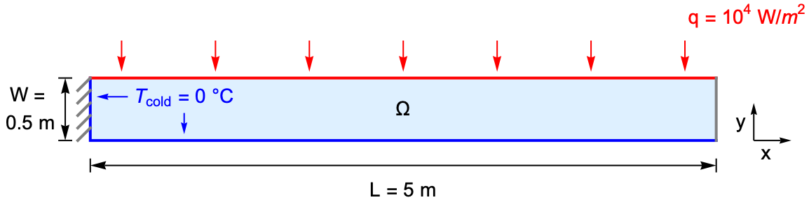
Thermal stress is a type of stress induced by a temperature change, which can lead to fracture or deformation of an object. In the following model a steel beam is fixed at the left and heated by a constant inward heat flux on the top surface. The left and the lower surfaces are kept at while the right end is assumed to be thermally insulated.

During the heating process the temperature on the top surface will be gradually increased. The resulting temperature gradient will then generate thermal stress and bend the beam downwards.

The evolution of the temperature field and the thermally induced deformation are simulated by sequentially the heat transfer and the structural mechanics models. The location and values of horizontal and vertical displacement will then be calculated.

The symbols and corresponding units used here are summarized in the Nomenclature section.

Please refer to the information provided in "Heat Transfer" for a more general theoretical background for heat transfer analysis.

Load the finite element package.

Multiphysics Model

There are two physical domains involved in this application: the heat transfer model and the structural mechanics model. The coupling between two models is one-way since only the structural deformation depends on the temperature but the temperature field does not depend on the deformation of the object in this model. This type of problem is considered as a sequential multiphysics model, and will be solved in two steps.

First the heat transfer model is built to simulate the temperature field of the beam. The structural mechanics model is then constructed and uses the temperature field previously computed to show the thermally induced deformation. This is what is called a sequential simulation and is possible because the deformation of the object does not couple back and influence the thermal distribution. Sequential models are possible when there is a coupling that is one directional. An alternative approach is to model both the temperature field and the deformation in a single PDE model. We then speak of a fully coupled model.

In this approach, we first consider the heat equation and then the solid mechanics equation.

Heat Transfer Model

The heat equation (1) is used to solve for the temperature field in a heat transfer model:

For a transient heat transfer model without sources, the source term in (2) is set to zero. Since a solid is modeled, any internal velocity also vanishes and the heat equation simplifies to:

Set up a 2D transient heat transfer model.

Structural Mechanics Model

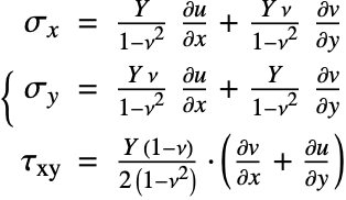
In structural mechanics, the plane stress relation (3) describes the deformation of thin objects. Here, "thin" means thin relative to the other dimensions of the object. The two dependent variables , denote the deformation in and directions, respectively. As material data, Young's modulus and the Poisson ratio need to be specified.

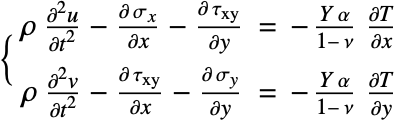
The equilibrium equation (4), which denotes the force balance in the and directions, is then used as the governing PDE of the structural mechanics model. On the right hand side and model any external force that may act on the object.

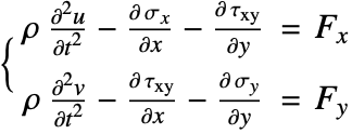
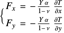
In this model the temperature-induced thermal load is the only external force that applies on the beam, and is coupled to the plane-stress PDE (5) as the source term on the right hand side. The magnitude of the thermal load , is related to the temperature and the thermal expansion coefficient by the thermal stress equation:

Define a transient plane stress operator.

Set up material parameters for the steel beam.

Here

is the density ,
is the heat capacity ,
is the thermal conductivity ,
is the Young's modulus ,
is the thermal expansion coefficient ,
is the Poisson ratio.

Set up the model parameters.

Domain

The steel beam to be modeled has a length of and a width of .

Define the 2D domain

In order to get a good result, a finer than the default grid is applied for the mesh generation. Here the maximum grid size is set to so that about one thousand elements are used.

Discretize the domain with a prescribed mesh size.

Solve the PDE Model

In the following section the heat transfer model will be solved first to simulate the temperature field of the beam. The structural mechanics model is then constructed to show the thermally induced deformation.

Heat Transfer Model

At the beginning of the simulation, the temperature of the steel beam is set to the temperature .

Set up the initial temperature of the beam.

The left and bottom surfaces are kept at the initial temperature at all time.

Set up a temperature surface boundary condition on the lower and bottom boundaries.

The top surface of the beam is subjected to a constant inward heat flux .

Set up the heat flux boundary condition on the top surface.

Specify the heat transfer PDE with the model parameters.

Define the simulation end time and solve the heat transfer model.

To inspect the heat flow within the steel beam, we visualize the temperature distribution evolving in time.

Set up a legend bar and ContourPlot options for the temperature field plot.

Visualize the temperature field.

See this note about improving the visual quality of the animation.

Due to the inward heat flux on the top surface, the temperature difference across the beam has been risen to in less then three hours ().

With the temperature profile in hand we can calculate the corresponding thermal load on the beam. The beam deformation is then solved by the structural mechanics model in the following section.

Structural Mechanics Model

In this model the temperature-induced thermal load is the only external force that applies on the beam, and is coupled to the plane-stress PDE (6) as the source term on the right hand side. The magnitude of the thermal load , is related to the temperature and the thermal expansion coefficient by the thermal stress equation:

Set up the initial condition to denote an undeformed beam at

On the left-hand side of the beam, the deformation variables , are held fixed with zero displacement.

Set up the boundary conditions so that the beam is held fixed at the left.

Specify the structural mechanics PDE with the model parameters and replace the symbolic

with the thermal simulation result

Solve the structural mechanics model and monitor the time/memory usage.

To inspect the effect of the thermal loading, the following visualization combines the resulting structural deformation with the temperature field.

Post-processing and Visualization

In order to show the structural deformation, the deformed element mesh is created for the beam based on the interpolating functions given.

Create an InterpolatingFunction for a time

Extract the undeformed boundary mesh wireframe as a comparison.

Define a help function TempDeformPlot to efficiently generate the temperature-structural plot at each time step.

Note that the deformation is scaled by a factor of to better demonstrated the result.

Visualize the scaled deformation and the temperature field of the steel beam.

See this note about improving the visual quality of the animation.

Next, to find the maximum beam deformation the components , are visualize with contour plots.

Set up a legend bar and ContourPlot options for the visualization.

In order to show the final deformation of the beam, the deformed element mesh and the resulting interpolating functions are set up at the simulation end time: .

Set up the deformed mesh and interpolating functions on the deformed mesh.

Visualize the scaled deformation in the

and

directions.

It is seen that the largest deformation of the beam occurs at the upper right corner. The maximum , values can be retrieved to show the exact deformation amount in both and directions.