InhomogeneousPoissonProcess


InhomogeneousPoissonProcess
InhomogeneousPoissonProcess[λ[t],t]
表示非齐次泊松过程,其中强度 λ[t] 是 t 的函数.
更多信息
- InhomogeneousPoissonProcess 是一个连续时间离散状态的过程.
- InhomogeneousPoissonProcess 在时间 t 是区间 0 到 t 的事件数.
- 区间 0 到 t 间的事件数遵循带有均值
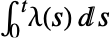 的 PoissonDistribution.
- InhomogeneousPoissonProcess 定义中的强度函数 λ[t] 被假设为有效的. 尤其是,它被认为是 t 的连续的、正值函数.
- InhomogeneousPoissonProcess 可与函数 Mean、PDF、Probability 和 RandomFunction 一起使用.
范例
打开所有单元 关闭所有单元基本范例 (3)
data = RandomFunction[InhomogeneousPoissonProcess[2 + 1 / (1 + t ^ 2), t], {0, 20}];ListStepPlot[data, Filling -> Axis]Mean[InhomogeneousPoissonProcess[2 + 1 / (1 + t ^ 2), t][t]]Variance[InhomogeneousPoissonProcess[2 + 1 / (1 + t ^ 2), t][t]]CovarianceFunction[InhomogeneousPoissonProcess[2 + t ^ 2, t], s, w]Plot3D[Evaluate@CovarianceFunction[InhomogeneousPoissonProcess[2 + t ^ 2, t], s, w], {s, 1, 10}, {w, 1, 10}, ColorFunction -> "Rainbow", PlotRange -> All, AxesLabel -> Automatic]范围 (10)
基本用途 (5)
data = RandomFunction[InhomogeneousPoissonProcess[(2 + Sin[t]) / 4, t], {0, 35}, 4]ListStepPlot[data, Filling -> Axis]RandomFunction[InhomogeneousPoissonProcess[2 + 1 / (1 + t ^ 2), t], {4}, WorkingPrecision -> 20]["Path"]f1[t_] = t;
f2[t_] = 2 + 1 / (1 + t ^ 2);
f3[t_] = (3 + Cos[t]) / 7;sample := (SeedRandom[3];RandomFunction[InhomogeneousPoissonProcess[#[t], t], {10}]&);ListStepPlot[sample[#], Filling -> Axis, PlotLabel -> #]& /@ {f1, f2, f3}CorrelationFunction[InhomogeneousPoissonProcess[2 + t, t], s1, s2]Simplify[%, s1 < s2]AbsoluteCorrelationFunction[InhomogeneousPoissonProcess[Cos[t] + 2, t], s1, s2]Simplify[%, s1 < s2]过程切片性质 (5)
单变量 SliceDistribution:
DiscretePlot[Evaluate@Table[PDF[InhomogeneousPoissonProcess[2 + 1 / (1 + τ ^ 2), τ][t], x], {t, times = {1, 4, 8}}], {x, 0, 30}, PlotLegends -> ("t = " ~~ ToString[#]& /@ times)]InhomogeneousPoissonProcess[2 + 1 / (1 + t ^ 2), t][t]PDF[InhomogeneousPoissonProcess[2 + 1 / (1 + t ^ 2), t][t], x]SliceDistribution[InhomogeneousPoissonProcess[2 + 1 / (1 + t ^ 2), t], {1, 3, 7}]//Mean更高阶 PDF:
PDF[InhomogeneousPoissonProcess[2 + 1 / (1 + t ^ 2), t][{1, 3, 7}], {x, y, z}]Expectation[x + E ^ (-x), xInhomogeneousPoissonProcess[2 + t, t][t]]Probability[x[t] ^ 2 < t - 1, xInhomogeneousPoissonProcess[2 + t, t]]𝒫 = InhomogeneousPoissonProcess[2 + 1 / (1 + t ^ 2), t];Moment[𝒫[t], r]CharacteristicFunction[𝒫[t], w]MomentGeneratingFunction[𝒫[t], w]CentralMoment 对于符号阶数没有解析式:
CentralMoment[𝒫[t], r]CentralMoment[𝒫[t], 4]CentralMomentGeneratingFunction[𝒫[t], w]FactorialMoment 与其母函数:
FactorialMoment[𝒫[t], r]FactorialMomentGeneratingFunction[𝒫[t], w]Cumulant 与其母函数:
Cumulant[𝒫[t], r]CumulantGeneratingFunction[𝒫[t], w]Covariance[InhomogeneousPoissonProcess[2 + t, t][{1, 2, 3}]]N[%]//MatrixFormCovariance[RandomVariate[InhomogeneousPoissonProcess[2 + t, t][{1, 2, 3}], 10 ^ 4]]//N//MatrixForm应用 (3)
arrivalrates = {{0, 8}, {1, 9}, {2, 7}, {4, 6}, {5, 12}, {6, 14}, {7, 11}, {8, 6}, {9, 4}, {10, 3}, {11, 8}, {12, 15}, {13, 12}, {14, 10}, {15, 8}, {16, 6}, {17, 12}, {18, 17}, {19, 15}, {20, 12}, {21, 6}, {22, 5}, {23, 7}};λ[t_] = Interpolation[arrivalrates, InterpolationOrder -> 1][t];Plot[λ[t], {t, 0, 23}, Exclusions -> None, Filling -> Axis]𝒫 = InhomogeneousPoissonProcess[λ[t], t];NProbability[x > 200, x𝒫[23]]data = RandomFunction[𝒫, {0, 23, 1}, 4];ListStepPlot[data]sim = RandomFunction[𝒫, {0., 23, 1}, 10 ^ 3];
slopes = Map[# / 23.&, sim["LastValues"]];
Mean[slopes]𝒫 = TransformedProcess[p[t] ^ 2, pInhomogeneousPoissonProcess[2 + 1 / (1 + t ^ 2), t], t];data = RandomFunction[𝒫, {0, 30, 1}, 3]ListStepPlot[data]Mean[𝒫[t]]Variance[𝒫[t]]带有韦伯失败率密度的非齐次泊松过程是众所周知的韦伯泊松过程:
λ[α_, β_, t_] = Refine[HazardFunction[WeibullDistribution[α, β], t], t > 0]WeibullPoissonProcess = InhomogeneousPoissonProcess[λ[2 / 3, 1 / 2, t], t]paths = RandomFunction[WeibullPoissonProcess, {0, 30}, 6, Method -> "Direct"]ListStepPlot[paths]sim = RandomFunction[WeibullPoissonProcess, {0, 30}, 10 ^ 3, Method -> "Direct"];
slopes = Map[# / 30.&, sim["LastValues"]];
Mean[slopes]NIntegrate[λ[2 / 3, 1 / 2, t], {t, 0, 30}] / 30属性和关系 (3)
InhomogeneousPoissonProcess 是一个跳跃过程:
path = RandomFunction[InhomogeneousPoissonProcess[2 + 1 / (1 + t ^ 2), t], {0, 10}];
f = path["PathFunction"];
jumps = path["Times"];Plot[f[t], {t, 0, 10}, Exclusions -> jumps, ExclusionsStyle -> Red]WeakStationarity[InhomogeneousPoissonProcess[2 + 1 / (1 + t ^ 2), t]]Mean[InhomogeneousPoissonProcess[2 + 1 / (1 + t ^ 2), t][t]]带有常密度的非齐次泊松过程是 PoissonProcess:
ipp = InhomogeneousPoissonProcess[λ, t];pp = PoissonProcess[λ];Mean /@ {ipp[t], pp[t]}Variance /@ {ipp[t], pp[t]}PDF[#, x]& /@ {ipp[t], pp[t]}CovarianceFunction[#, s, t]& /@ {ipp, pp}PDF[#, {x, y}]& /@ {ipp[{s, t}], pp[{s, t}]}可能存在的问题 (1)
λ[t_] = Abs[Tan[t]] + 1;
Plot[λ[t], {t, 0, 3}, PlotRange -> All]𝒫 = InhomogeneousPoissonProcess[λ[t], t];TimeConstrained[RandomFunction[𝒫, {0, 3}], 1]TimeConstrained[RandomFunction[𝒫, {0, 3}, Method -> "Thinning"], 1]RandomFunction[𝒫, {0, 3}, Method -> "Inversion"]RandomFunction[𝒫, {0, 3}, Method -> "Direct"]ListLinePlot[%, PlotRange -> All]巧妙范例 (1)
SeedRandom[34];𝒫 = InhomogeneousPoissonProcess[1.1 + Sin[t] / (1 + t ^ 2), t];
data = RandomFunction[𝒫, {0, 50}, 300];sd = data["SliceData", 50];cf = ColorData["Rainbow"];
sliced = BarChart[Last[#], Axes -> False, BarOrigin -> Left, AspectRatio -> 4, ChartStyle -> (cf /@ Rescale[MovingAverage[First[#], 2], {Min[sd], Max[sd]}, {0, 1}]), ImageSize -> 43]&[HistogramList[sd, {Range[Min[sd], Max[sd], (Max[sd] - Min[sd]) / 20]}]];ListLinePlot[data, ImageSize -> 400, PlotRange -> All,
AspectRatio -> 3 / 4, Epilog -> Inset[sliced, {50.5, 57}, {0, 10.5}], PlotStyle -> (cf /@ Rescale[sd]), BaseStyle -> Thin, PlotRangePadding -> {{0, 20}, {.5, 7}}]
Wolfram Research (2015),InhomogeneousPoissonProcess,Wolfram 语言函数,https://reference.wolfram.com/language/ref/InhomogeneousPoissonProcess.html.
文本
Wolfram Research (2015),InhomogeneousPoissonProcess,Wolfram 语言函数,https://reference.wolfram.com/language/ref/InhomogeneousPoissonProcess.html.
CMS
Wolfram 语言. 2015. "InhomogeneousPoissonProcess." Wolfram 语言与系统参考资料中心. Wolfram Research. https://reference.wolfram.com/language/ref/InhomogeneousPoissonProcess.html.
APA
Wolfram 语言. (2015). InhomogeneousPoissonProcess. Wolfram 语言与系统参考资料中心. 追溯自 https://reference.wolfram.com/language/ref/InhomogeneousPoissonProcess.html 年