

ModelPredictiveController
ModelPredictiveController[sspec,cost,cons]
computes the model predictive controller for the system specification sspec that minimizes the cost function cost and satisfies the constraints cons.
ModelPredictiveController[…,"prop"]
returns the value of the property "prop".
Details and Options
- Model predictive control is also known as MPC.
- A model predictive controller is computed by minimizing a cost function of state and control input over a finite horizon while allowing for constraints on both inputs and states. These constraints are often important to guarantee that the controller can be implemented safely.
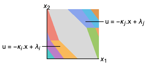
- The resulting controller has a simple piecewise affine form
 , where
  is the feedback control input and
  is the state of the system. These can easily be deployed in microcontrollers and used for fast processes.
 - A regulator aims to maintain the system at an equilibrium position despite disturbances
 pushing it away. Typical examples include maintaining an inverted pendulum in its upright position or maintaining an aircraft in level flight.
 - The MPC regulator is specified as the feedback that minimizes the cost
 subject to the system dynamics
  in sspec and constraints cons. The cost
  becomes small when both state
  and feedback control input
  become small.
 -

1-norm, weighted integral absolute error (IAE) 
squared 2-norm, weighted integral squared error (ISE) or weighted "energy" 
 -norm, weighted peak value
 - The cost
 is specified in the cost Association with the following keys:
 -
η "Horizon" integer time horizon q "StateWeight" matrix cost on states r "InputWeight" matrix cost on inputs p "StateInputWeight" matrix cost on cross-coupled states and inputs m "Norm" 1, 2 or 
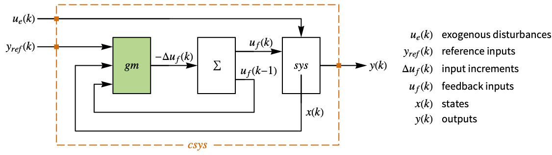
- A tracker aims to track reference signals
 despite disturbances
  . Typical examples include a cruise control system for a car or path tracking for a robot.
 - The MPC tracker is specified as the feedback that minimizes a cost subject to the system dynamics
 in sspec and constraints cons. The cost becomes small when both predicted error
  and the incremental feedback control input
  become small.
 -

1-norm, weighted integral absolute error (IAE) 
squared 2-norm, weighted integral squared error (ISE) or weighted "energy" 
 -norm, weighted peak value
 - The terms in the cost function expressions are the following:
-
η "Horizon" integer time horizon qe "ErrorWeight" matrix cost on errors 
"InputIncrementWeight" matrix cost on input increments peΔ "ErrorInputIncrementWeight" matrix cost on cross coupled errors and input increments m "Norm" 1, 2 or 
- The constraints cons for both the regulator and tracker problems are formulated in terms of the state variables x, input variables u and output variables y. These can be defined using StateSpaceModel[{a,b,c,d},x,u,y,…].
- Constraints that hold for a particular time instant
 where
where  :
: -
xmin<=xi[k]<=xmax constraint on the value at time 
Δxmin<=xi[k2]-xi[k1]<=Δxmax constraint on the increment from time  to time
- Constraints that hold for all time instants k where
 :
: -
xmin<=xi<=xmax constraint on the value for all k min<=α1.x1+…+αn.xn+β<=max constraint on a linear combination for all k xminxxmax constraint on all the values for all k - The weight matrices
 ,
,  and
and  can be specified as follows:
 -
q constant weights {q,…,q,q} {{q},qη} varying end weight {q,…,q,qη} {q0,q1,…,qη} varying weights {q0,q1,…,qη} - ModelPredictiveController works for discrete-time linear systems that can be specified using StateSpaceModel[…,SamplingPeriodτ].
- The system specification sspec can have the following forms:
-
StateSpaceModel[…] linear control input and linear state AffineStateSpaceModel[…] linear control input and nonlinear state NonlinearStateSpaceModel[…] nonlinear control input and nonlinear state SystemModel[…] general system model <…> detailed system specification given as an Association - The detailed system specification can have the following keys:
-
"InputModel" sys any one of the models "FeedbackInputs" All the feedback inputs uf "TrackedOutputs" None the tracked outputs yref - The feedback inputs can have the following forms:
-
{num1,…,numn} numbered inputs numi used by StateSpaceModel, AffineStateSpaceModel and NonlinearStateSpaceModel {name1,…,namen} named inputs namei used by SystemModel All uses all inputs - ModelPredictiveController returns a SystemsModelControllerData object cd that can be used to extract additional properties using the form cd["prop"].
- ModelPredictiveController[…,"prop"] can be used to directly get the value of cd["prop"].
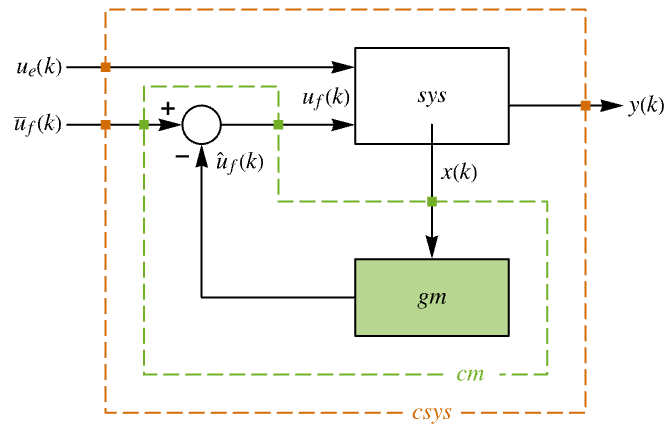
- Closed-loop system properties:
-
"BlockDiagram" block diagram of csys "ClosedLoopPoles" poles of the linearized "ClosedLoopSystem" "ClosedLoopSystem" system csys {"ClosedLoopSystem",cspec} detailed control over the form of the closed-loop system "ControllerModel" model cm "FeedbackGains" gain matrix κ or its equivalent "FeedbackGainsModel" model gm "FeedbackRegions" regions from which the feedback is feasible "OptimalCost" optimal value of 
"QuasiClosedLoopSystem" closed-loop assembled with "QuasiFeedbackGains" "QuasiFeedbackGains" feedback gains that depend only on initial values "QuasiFeedbackGainsModel" systems model of "QuasiFeedbackGains" - Infinite horizon problem properties:
-
"MaximalLQRInvariantRegion" maximal region  with LQR feedback gains
"MaximalStabilizableRegion" maximal region ![K_infty TemplateBox[{{(, O}, infty, LQR}, Subsuperscript])](Files/ModelPredictiveController.en/41.png "K_infty TemplateBox[{{(, O}, infty, LQR}, Subsuperscript])") that can be steered into
that can be steered into 
"MinimalFiniteHorizon" minimal horizon at which states in ![K_infty TemplateBox[{{(, O}, infty, LQR}, Subsuperscript])](Files/ModelPredictiveController.en/43.png "K_infty TemplateBox[{{(, O}, infty, LQR}, Subsuperscript])") enter
enter 
- Basic design properties:
-
"Design" type of controller design "DesignModel" model used for the design "DesignModelSamplingMethod" sampling method used to obtain "DesignModel" "DesignModelSamplingPeriod" sampling period of "DesignModel" "Horizon" horizon η "Norm" 1-, squared 2-, or ∞-norm - Input model properties:
-
"FeedbackInputs" inputs uf of sys used for feedback "InputModel" input model sys "InputsCount" number of inputs u of sys "OpenLoopPoles" poles of "DesignModel" "OutputsCount" number of outputs y of sys "SamplingPeriod" sampling period of sys "StatesCount" number of states x of sys "TrackedOutputs" outputs yt of sys that are tracked
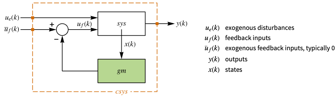
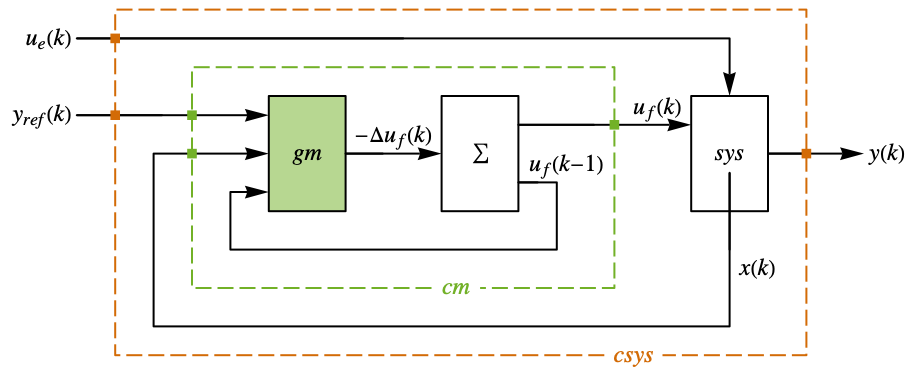
The diagram of the regulator layout.
The diagram of the tracker layout.
Examples
open all close allBasic Examples (2)
Solve the infinite horizon regulator problem for a system with states {x1,x2} and control input u:
ssm = StateSpaceModel[{{{1, 1}, {0, 1}}, {{0}, {1}}}, {Subscript[x, 1], Subscript[x, 2]}, u, SamplingPeriod -> 1]cost = <|"Horizon" -> Infinity, "StateWeight" -> IdentityMatrix[2], "InputWeight" -> {{0.1}}|>;And the state and input constraints:
cons = -3 ≤ Subscript[x, 1] ≤ 3∧-3 ≤ Subscript[x, 2] ≤ 3∧-1 ≤ u ≤ 1;Compute the resulting MPC controller:
cd = ModelPredictiveController[ssm, cost, cons]csys = cd["ClosedLoopSystem"]The regions with feasible feedback:
reg = cd["FeedbackRegions"];
regPlot = RegionPlot[Evaluate[List@@reg[[1]]], {Subscript[x, 1], -3, 3}, {Subscript[x, 2], -3, 3}, PlotPoints -> 20, MaxRecursion -> 5]
The simulation of the closed-loop system from different initial points in the feasible region:
Table[Arrow[OutputResponse[{csys, <|1 -> RandomPoint[reg]|>},
PadRight[{0}, 6]]], 12];
Show[regPlot, Graphics[%]]Solve the finite horizon regulator problem for a system with states {x1,x2} and control input u:
ssm = StateSpaceModel[{{{1, 1}, {0, 1}}, {{1}, {0.5}}}, {Subscript[x, 1], Subscript[x, 2]}, u, SamplingPeriod -> 0.1]cost = <|"Horizon" -> 4, "StateWeight" -> DiagonalMatrix[{0.5, 0}], "InputWeight" -> {{0.5}}|>;And the state and input constraints:
cons = -5 ≤ Subscript[x, 1] ≤ 5∧-5 ≤ Subscript[x, 2] ≤ 5∧-1 ≤ u ≤ 1;Compute the resulting MPC controller:
cd = ModelPredictiveController[ssm, cost, cons]csys = cd["ClosedLoopSystem"]The response of the closed-loop system to an input sequence:
OutputResponse[csys, Table[PadRight[{0.1, 0, -0.1, 0, 0, 0.1}, 20], 2]];
ListStepPlot[%, PlotRange -> All, DataRange -> {0, 0.1 20}]osys = cd["QuasiClosedLoopSystem"]The response of the quasi closed-loop system to an input sequence:
OutputResponse[{osys, <|1 -> {0.1, 0.1}|>}, Table[PadRight[{0}, 10], 2]];
ListStepPlot[%, PlotRange -> All, DataRange -> {0, 0.1 10}]
Scope (43)
Basic Uses (5)
Solve the regulator problem for a discrete-time system with states {x1,x2} and control input u:
ssm = StateSpaceModel[{{{1, -1}, {0, 1}}, {{0}, {1}}}, {Subscript[x, 1], Subscript[x, 2]}, u, SamplingPeriod -> 1]cost = <|"Horizon" -> 3, "StateWeight" -> IdentityMatrix[2], "InputWeight" -> {{0.1}}|>;Constrain the states ![]() and the control input
and the control input ![]() :
:
cons = -2 ≤ Subscript[x, 1] ≤ 2∧-3 ≤ Subscript[x, 2] ≤ 3∧-1 ≤ u ≤ 1;cd = ModelPredictiveController[ssm, cost, cons]csys = cd["ClosedLoopSystem"]The response of the closed-loop system:
or = OutputResponse[csys, PadRight[{0, 0.8}, 20]];
ListStepPlot[or, PlotRange -> All]
The closed-loop system from above:
csys = SystemsConnectionsModel[{StateSpaceModel[{{{1, -1}, {0, 1}}, {{0}, {1}}},
   {Subscript[x, 1], Subscript[x, 2]}, u, SamplingPeriod -> 1],
  DiscreteInputOutputModel[Association["SampledSeries" -> TemporalData[TimeSeries,
      {{{Piecewise[{{{1. ... a", "TimePath", "Times", "TimeSeries", "TimeValues", "Type",
    "Values"}], StateSpaceModel[{{}, {}, {}, {{1, -1}}}, SamplingPeriod -> 1]},
 {{3, 1} -> {1, 1}, {1, 1} -> {2, 1}, {1, 2} -> {2, 2}, {2, 1} -> {3, 2}}, {{3, 1}},
 {{1, 1}, {1, 2}}];
It consists of the input model, feedback gains and comparator:
subSys = First[List@@csys]SystemsModelOrder /@ subSysSimulate the closed-loop system from a nonzero initial condition:
OutputResponse[{csys, <|1 -> {1, -1}|>}, PadRight[{0, 0.8}, 20]];
ListStepPlot[%, PlotRange -> All]
Start from a different initial condition:
OutputResponse[{csys, <|1 -> {-0.1, 1}|>}, PadRight[{0, 0.8}, 20]];
ListStepPlot[%, PlotRange -> All]
A multiple-input system with inputs {u1,u2}:
ssm = StateSpaceModel[{{{1, 0}, {1, 1}}, {{1.0, 0}, {0, 1.0}}}, {Subscript[x, 1], Subscript[x, 2]}, {Subscript[u, 1], Subscript[u, 2]}, SamplingPeriod -> 1]cost = <|"Horizon" -> 3, "StateWeight" -> IdentityMatrix[2], "InputWeight" -> 2 IdentityMatrix[2]|>;cons = -1 ≤ Subscript[x, 1] ≤ 1∧-1 ≤ Subscript[x, 2] ≤ 1∧-0.5 ≤ Subscript[u, 1] ≤ 0.5∧-0.5 ≤ Subscript[u, 2] ≤ 0.5;cd = ModelPredictiveController[ssm, cost, cons]The controller is a DiscreteInputOutputModel:
fg = cd["FeedbackGainsModel"]It is essentially a series of piecewise functions:
Head /@ fg["Values"]And has the two states as inputs:
fg["InputVariables"]A system with sampling period of 0.1:
ssm = StateSpaceModel[{{{0, 1.}, {-1, -0.1}}, {{0}, {1}}}, {Subscript[x, 1], Subscript[x, 2]}, {u}, SamplingPeriod -> 0.1]cost = <|"Horizon" -> 3, "StateWeight" -> IdentityMatrix[2], "InputWeight" -> {{0.1}}|>;cons = -1 ≤ Subscript[x, 1] ≤ 1∧-1 ≤ Subscript[x, 2] ≤ 1∧-0.5 ≤ u ≤ 0.5;cd = ModelPredictiveController[ssm, cost, cons]or = OutputResponse[cd["ClosedLoopSystem"], PadRight[{0, -0.3, 0, 0.5}, 12]]Plot the response at the sampling instants:
ListStepPlot[or, PlotRange -> All]Plot it as a function of time:
ListStepPlot[or, PlotRange -> All, DataRange -> {0, 0.1 12}]The controller data object from above:
cd = SystemsModelControllerData[«2»];Compute the controller effort by first obtaining the controller model and closed-loop system:
{cm, csys} = cd[{"ControllerModel", "ClosedLoopSystem"}]The output response to an input sequence:
inp = PadRight[{0, -0.3, 0, 0.5}, 12];
or = OutputResponse[cd["ClosedLoopSystem"], inp]
The controller effort along with the control bounds ![]() :
:
OutputResponse[cm, Join[{inp}, or]]
ListStepPlot[Join[%, Table[{-0.5, 0.5}, 12]], IconizedObject[«plotOpts»]]Norm (4)
Compute a controller that minimizes a 1-normed cost:
cost = <|"Norm" -> 1, "Horizon" -> 3, "StateWeight" -> DiagonalMatrix[{1, 1}], "InputWeight" -> {{1}}|>;
cd = ModelPredictiveController[IconizedObject[«ssm»], cost, IconizedObject[«cons»]]
The controller is a DiscreteInputOutputModel:
fgm = cd["FeedbackGainsModel"]It is a series of piecewise functions:
MapAt[Head, fgm["Path"], {All, 2}]Compute a controller that minimizes a ![]() -normed cost:
-normed cost:
cost = <|"Norm" -> ∞, "Horizon" -> 3, "StateWeight" -> DiagonalMatrix[{1, 1}], "InputWeight" -> {{1}}|>;
cd = ModelPredictiveController[IconizedObject[«ssm»], cost, IconizedObject[«cons»]]
The controller is a DiscreteInputOutputModel:
fgm = cd["FeedbackGainsModel"]It is a series of piecewise functions:
MapAt[Head, fgm["Path"], {All, 2}]Compute a controller that minimizes a squared 2-normed cost:
cost = <|"Norm" -> 2, "Horizon" -> 3, "StateWeight" -> DiagonalMatrix[{1, 1}], "InputWeight" -> {{1}}|>;
cd = ModelPredictiveController[IconizedObject[«ssm»], cost, IconizedObject[«cons»]]
The controller is a DiscreteInputOutputModel:
fgm = cd["FeedbackGainsModel"]It is a series of piecewise functions:
MapAt[Head, fgm["Path"], {All, 2}]Compute a controller that minimizes a squared 2-normed cost for an infinite horizon:
cost = <|"Norm" -> 2, "Horizon" -> ∞, "StateWeight" -> DiagonalMatrix[{1, 1}], "InputWeight" -> {{1}}|>;
cd = ModelPredictiveController[IconizedObject[«ssm»], cost, IconizedObject[«cons»]]
The controller is a NonlinearStateSpaceModel:
Head[fgm = cd["FeedbackGainsModel"]]SystemsModelOrder[fgm]And is a piecewise function of the states of the input model:
cd["InputModel"][[2]]Plot3D[cd["FeedbackGains"], {x1, -5, 5}, {x2, -5, 5}]Tracking (4)
Solve the tracking problem for a discrete-time system with states {x1,x2} and control input u:
ssm = StateSpaceModel[{{{1, 1}, {0, 1}}, {{1}, {0.45}}, {{1, 0}}}, {Subscript[x, 1], Subscript[x, 2]}, u, SamplingPeriod -> 1]cost = <|"Horizon" -> 4, "ErrorWeight" -> {{10}}, "InputIncrementWeight" -> {{1}}|>;cons = -5 ≤ Subscript[x, 1] ≤ 5∧-5 ≤ Subscript[x, 2] ≤ 5∧-1 ≤ u ≤ 1;Compute the tracking controller:
cd = ModelPredictiveController[ssm, cost, cons]csys = cd["ClosedLoopSystem"]OutputResponse[csys, PadRight[{1, 2, 3}, 20, 2]];
ListStepPlot[%, PlotRange -> All]A block diagram of the closed-loop system:
cd["BlockDiagram"]The closed-loop system from above:
csys = SystemsConnectionsModel[«4»];Its response to a nonconstant step-like reference signal:
ref = Splice[ConstantArray[#, 10]]& /@ {2, 4, 8};
or = OutputResponse[csys, ref][[1]]
The response does not exceed the upper limit of 5:
ListStepPlot[{ref, or}, PlotRange -> All, PlotLegends -> {"ref.", "act."}]The response to a sinusoidal reference:
ref = Table[Sin[t], {t, 0, 10, 0.1}];or = OutputResponse[csys, ref];ListStepPlot[{ref, or[[1]]}, PlotRange -> All, PlotLegends -> {"ref.", "act."}]Compare the responses with different norms:
TableForm[cost = Table[<|"Norm" -> m, "Horizon" -> 3, "ErrorWeight" -> {{10}}, "InputIncrementWeight" -> {{1}}|>, {m, {2, 1, Infinity}}]]The controllers for the different norms:
cd = Table[ModelPredictiveController[IconizedObject[«ssm»], i, IconizedObject[«cons»]], {i, cost}]csys = Table[i["ClosedLoopSystem"], {i, cd}]ref = PadRight[{1, 0, 2, 1, 3}, 20, 2];or = Table[OutputResponse[i, ref][[1]], {i, csys}];
ListStepPlot[or, PlotRange -> All, PlotLegends -> {2, 1, Infinity}]The responses of the 1- and ![]() -norm are the same because it is a single input and single output system:
-norm are the same because it is a single input and single output system:
Differences[or[[2 ;; 3]]]The error norms of the 2- and 1-norm responses:
Thread[{2, 1} -> Table[Norm[ref - i], {i, or[[1 ;; 2]]}]]Compare the norms for a multiple-output system:
ssm = StateSpaceModel[{{{1, 1}, {0, 1}}, {{1}, {0.1}}}, {Subscript[x, 1], Subscript[x, 2]}, {u}, SamplingPeriod -> 1, SystemsModelLabels -> None]The cost specifications for the different norms:
TableForm[cost = Table[<|"Norm" -> m, "Horizon" -> 3, "ErrorWeight" -> DiagonalMatrix[{10, 5}], "InputIncrementWeight" -> {{1}}|>, {m, {2, 1, Infinity}}]]cd = Table[ModelPredictiveController[ssm, i, IconizedObject[«cons»]], {i, cost}]csys = Table[i["ClosedLoopSystem"], {i, cd}]or = Table[OutputResponse[i, PadRight[{1, 0, 2, 1, 3}, 40, 2]][[1]], {i, csys}];
ListStepPlot[or, PlotRange -> All, PlotLegends -> {2, 1, Infinity}]The difference between the responses of the 1- and ![]() -norm costs:
-norm costs:
ListStepPlot[Differences[or[[2 ;; 3]]]]Plant Models (8)
The controller for a system specified as a StateSpaceModel:
ModelPredictiveController[StateSpaceModel[{{{0.1, 0}, {1, -0.1}}, {{0}, {1}}, {{1, 0}}, {{0}}},
 {Subscript[x, 1], Subscript[x, 2]}, {u},
 SamplingPeriod -> 1, SystemsModelLabels -> None], IconizedObject[«cost»], IconizedObject[«cons»]]
A system specified as an AffineStateSpaceModel:
assm = AffineStateSpaceModel[{{Cos[Subscript[x, 2]] + Sin[0.1*Subscript[x, 1]],
   Sin[Subscript[x, 1]] - Sin[0.1*Subscript[x, 2]]}, {{0}, {1}},
  {Subscript[x, 1]}, {{0}}}, {Subscript[x, 1],
Subscript[x, 2]}, {u}, {Automatic}, Automatic, SamplingPeriod -> 1];cd1 = ModelPredictiveController[assm, IconizedObject[«cost»], IconizedObject[«cons»]]It is computed based on a linear approximation:
cd2 = ModelPredictiveController[StateSpaceModel[assm], IconizedObject[«cost»], IconizedObject[«cons»]]The feedback gains are the same:
MatchQ[cd1["FeedbackGains"] - cd2["FeedbackGains"], {__ ? PossibleZeroQ}]A nonlinear system with nonzero operating points:
assm = AffineStateSpaceModel[{{Cos[Subscript[x, 2]] + Sin[0.1 Subscript[x, 1]], Sin[Subscript[x, 1]] - Sin[0.1 Subscript[x, 2]]}, {{0}, {1}}, {Subscript[x, 1]}}, {Subscript[x, 1] -> 0, Subscript[x, 2] -> 0.5 π}, {{u, Sin[0.05 π]}}, SamplingPeriod -> 1]cd1 = ModelPredictiveController[assm, IconizedObject[«cost»], IconizedObject[«cons»]]It is computed based on a linear approximation:
cd2 = ModelPredictiveController[StateSpaceModel[assm], IconizedObject[«cost»], IconizedObject[«cons»]]The nonzero operating points cause the gains to be different:
MatchQ[cd1["FeedbackGains"] - cd2["FeedbackGains"], {__ ? PossibleZeroQ}]A controller for a system specified as a NonlinearStateSpaceModel:
ModelPredictiveController[NonlinearStateSpaceModel[{{Sin[0.1*Subscript[x, 1]] +
    Sin[Subscript[x, 1]]*Subscript[x, 2],
   u - Sin[0.1*Subscript[x, 2]] + Subscript[x, 1]*
     Subscript[x, 2]}, {Subscript[x, 1]}},
 {Subscript[x, 1], Subscript[x, 2]}, {u}, {Automatic},
 Automatic, SamplingPeriod -> 1], IconizedObject[«cost»], IconizedObject[«cons»]]
A system specified as a continuous-time SystemModel:
sm = CreateSystemModel["exampleModel", {x'[t] + x[t] == u[t], y[t] == x[t]}, t, {"u"∈"Modelica.Blocks.Interfaces.RealInput", "y"∈"Modelica.Blocks.Interfaces.RealOutput"}]The complete system specification includes the sampling as well:
sspec = <|"InputModel" -> sm, "SamplingPeriod" -> 1|>;cost = <|"Horizon" -> 3, "StateWeight" -> {{5}}, "InputWeight" -> {{1}}|>;The constraints specified in terms of formal variables:
cons1 = -2 <= Subscript[, 1] <= 2∧-1 <= Subscript[, 1] <= 1;cd1 = ModelPredictiveController[sspec, cost, cons1]The constraints can also sometimes be specified using the variable labels:
SystemModelLinearize[sm]cons2 = -2 <= "x" <= 2∧-1 <= "u" <= 1;cd2 = ModelPredictiveController[sspec, cost, cons2]The feedback gains are the same:
MatchQ[cd1["FeedbackGains"] - cd2["FeedbackGains"], {__ ? PossibleZeroQ}]A system with feedback and exogenous inputs:
ssm = StateSpaceModel[{{{-0.2, 0.3}, {0, 1}}, {{0, 1}, {1, 1}}}, {Subscript[x, 1], Subscript[x, 2]}, {Subscript[u, 1], Subscript[u, 2]}, SamplingPeriod -> 0.1]The complete system specification:
sspec = <|"InputModel" -> ssm, "FeedbackInputs" -> 1|>;The cost includes only the feedback input cost:
cost = <|"Horizon" -> 5, "StateWeight" -> DiagonalMatrix[{1, 1}], "InputWeight" -> {{0.1}}|>;The constraints include only constraints on the feedback input:
cons = -1 ≤ Subscript[x, 1] ≤ 1∧-1 ≤ Subscript[x, 2] ≤ 1∧-1 ≤ Subscript[u, 1] ≤ 1;cd = ModelPredictiveController[sspec, cost, cons]The feedback gains model has the two states {x1,x2} as inputs and u1 as output:
SystemsModelDimensions[cd["FeedbackGainsModel"]]A system with multiple outputs:
ssm = StateSpaceModel[{{{-0.2, 0.3}, {0, 1}}, {{0}, {1}}, {{1, 0}, {0, 1}}}, {Subscript[x, 1], Subscript[x, 2]}, {u}, SamplingPeriod -> 0.1]The complete system specification to track only the first output:
sspec = <|"InputModel" -> ssm, "TrackedOutputs" -> 1|>;The cost includes only the error of the tracked output:
cost = <|"Horizon" -> 5, "ErrorWeight" -> {{1}}, "InputIncrementWeight" -> {{0.1}}|>;cons = -1 ≤ Subscript[x, 1] ≤ 1∧-1 ≤ Subscript[x, 2] ≤ 1∧ -1 ≤ u ≤ 1;cd = ModelPredictiveController[sspec, cost, cons]Only the first output is tracked:
cd["TrackedOutputs"]A SystemModel with multiple inputs:
sm = CreateSystemModel["exampleModel", {x''[t] + x'[t] + x[t] == u1[t] + u2[t], y[t] == x[t]}, t, {"u1"∈"Modelica.Blocks.Interfaces.RealInput", "u2"∈"Modelica.Blocks.Interfaces.RealInput", "y"∈"Modelica.Blocks.Interfaces.RealOutput"}];
sm["InputVariables"]
The feedback input specified using the variable names:
cd = ModelPredictiveController[<|"InputModel" -> sm, "SamplingPeriod" -> 0.1, "FeedbackInputs" -> "u1"|>, IconizedObject[«cost»], IconizedObject[«cons»]]cd["FeedbackInputs"]It is the first input of the linearized StateSpaceModel:
SystemModelLinearize[sm]Constraints (5)
The constraints specified as a logical expression:
cons = -1 ≤ Subscript[x, 1] ≤ 1∧-1 ≤ Subscript[x, 2] ≤ 1∧-2 ≤ u ≤ 2;ModelPredictiveController[IconizedObject[«ssm»], IconizedObject[«cost»], cons]The constraints specified as a list:
cons = {-1 ≤ Subscript[x, 1] ≤ 1, -1 ≤ Subscript[x, 2] ≤ 1, -2 ≤ u ≤ 2};
ModelPredictiveController[IconizedObject[«ssm»], IconizedObject[«cost»], cons]
The constraints specified with vector and scalar inequality constraints:
cons = -1{Subscript[x, 1], Subscript[x, 2]}1∧-2 ≤ u ≤ 2;
ModelPredictiveController[IconizedObject[«ssm»], IconizedObject[«cost»], cons]The constraints specified for specific ![]() :
:
cons = Join[Table[-1 ≤ Subscript[x, 1][k] ≤ 1, {k, 0, 3}], {-0.5 ≤ Subscript[x, 1][4] ≤ 0.5, -1 ≤ Subscript[x, 2] ≤ 1, -2 ≤ u ≤ 2}]cd = ModelPredictiveController[IconizedObject[«ssm»], IconizedObject[«cost»], cons]Constraints that include control rates:
cons = {-1 ≤ Subscript[x, 1] ≤ 1, -1 ≤ Subscript[x, 2] ≤ 1, -2 ≤ u ≤ 2, Splice@Table[-0.5 ≤ u[k + 1] - u[k] ≤ 0.5, {k, 0, 3}]}cd = ModelPredictiveController[IconizedObject[«ssm»], Association["Horizon" -> 5, "StateWeight" -> {{1, 0}, {0, 1}}, "InputWeight" -> {{0.1}}], cons]The response of the closed-loop system:
or = OutputResponse[{cd["ClosedLoopSystem"], <|1 -> {0.2, -0.1}|>}, Table[0, 10]];
ListStepPlot[%, DataRange -> {0, 10}, PlotRange -> All]ce = OutputResponse[cd["ControllerModel"], Join[{Table[0, 10]}, or]];
ListStepPlot[%, DataRange -> {0, 10}, PlotRange -> All]The control rates are in the limit ![]() :
:
Differences[ce[[1]]]Properties (17)
The list of available properties can be computed from the controller data object:
cd = ModelPredictiveController[StateSpaceModel[{{{0, 1.}, {0.09, 0}}, {{0}, {1}}, {{1, 0}}, {{0}}},
{Subscript[x, 1], Subscript[x, 2]}, {u},
SamplingPeriod -> 1, SystemsModelLabels -> None], <|"Horizon" -> 3, "StateWeight" -> {{10, 0}, {0, 1}}, "InputWeight" -> {{1}}|>, -1{Subscript[x, 1], Subscript[x, 2], u}1]cd["Properties"]A specific property can be computed directly:
ssm = StateSpaceModel[{{{0, 1}, {-0.21, 1}}, {{0}, {1}}, {{1, 0}}, {{0}}},
{Subscript[x, 1], Subscript[x, 2]}, {u},
SamplingPeriod -> 1, SystemsModelLabels -> None];
cost = <|"Horizon" -> 3, "StateWeight" -> {{10, 0}, {0, 1}}, "InputWeight" -> {{1}}|>;
cons = -1{Subscript[x, 1], Subscript[x, 2], u}1;ModelPredictiveController[ssm, cost, cons, "ClosedLoopSystem"]A list of properties can also be computed:
{csys, cm} = ModelPredictiveController[ssm, cost, cons, {"ControllerModel", "ClosedLoopSystem"}]fg = ModelPredictiveController[StateSpaceModel[{{{0, 1}, {-0.21, 1}}, {{0}, {1}}, {{1, 0}}, {{0}}},
{Subscript[x, 1], Subscript[x, 2]}, {u},
SamplingPeriod -> 1, SystemsModelLabels -> None], <|"Horizon" -> 3, "StateWeight" -> {{10, 0}, {0, 1}}, "InputWeight" -> {{1}}|>, -1{Subscript[x, 1], Subscript[x, 2], u}1, "FeedbackGains"]It is a series of piecewise functions:
Head /@ fgWhich are affine in the states:
First /@ First[#]& /@ fgIt can be used to compute the feedback gains model:
DiscreteInputOutputModel[fg, {Subscript[x, 1], Subscript[x, 2]}, SamplingPeriod -> 1]Obtain the feedback gains model directly:
fgm = ModelPredictiveController[StateSpaceModel[{{{0, 1}, {-0.21, 1}}, {{0}, {1}}, {{1, 0}}, {{0}}},
{Subscript[x, 1], Subscript[x, 2]}, {u},
SamplingPeriod -> 1, SystemsModelLabels -> None], <|"Horizon" -> 3, "StateWeight" -> {{10, 0}, {0, 1}}, "InputWeight" -> {{1}}|>, -1{Subscript[x, 1], Subscript[x, 2], u}1, "FeedbackGainsModel"]It can be used to compute the controller model:
cm = SystemsConnectionsModel[{StateSpaceModel[{{}, {}, {}, {{1, -1}}}, SamplingPeriod -> 1, SystemsModelLabels -> None], fgm}, {{2, 1} -> {1, 2}}, {{1, 1}, {2, 1}, {2, 2}}, {{1, 1}}]csys = SystemsConnectionsModel[{StateSpaceModel[{{{0, 1}, {-0.21, 1}}, {{0}, {1}}, {{1, 0}, {0, 1}}, {{0}, {0}}},
{Subscript[x, 1], Subscript[x, 2]}, {u}, Automatic,
SamplingPeriod -> 1, SystemsModelLabels -> None], fgm, StateSpaceModel[{{}, {}, {}, {{1, -1}}}, SamplingPeriod -> 1, SystemsModelLabels -> None]}, {{3, 1} -> {1, 1}, {1, 1} -> {2, 1}, {1, 2} -> {2, 2}, {2, 1} -> {3, 2}}, {{3, 1}}, {{1, 1}}]The block diagram of the closed-loop system:
ModelPredictiveController[StateSpaceModel[{{{0, 1}, {-0.21, 1}}, {{0}, {1}}, {{1, 0}}, {{0}}},
{Subscript[x, 1], Subscript[x, 2]}, {u},
SamplingPeriod -> 1, SystemsModelLabels -> None], <|"Horizon" -> 3, "StateWeight" -> {{10, 0}, {0, 1}}, "InputWeight" -> {{1}}|>, -1{Subscript[x, 1], Subscript[x, 2], u}1, "BlockDiagram"]optCost = ModelPredictiveController[StateSpaceModel[{{{0, 1}, {-0.21, 1}}, {{0}, {1}}, {{1, 0}}, {{0}}},
{Subscript[x, 1], Subscript[x, 2]}, {u},
SamplingPeriod -> 1, SystemsModelLabels -> None], <|"Horizon" -> 3, "StateWeight" -> {{10, 0}, {0, 1}}, "InputWeight" -> {{1}}|>, -1{Subscript[x, 1], Subscript[x, 2], u}1, "OptimalCost"];It is a sum of three piecewise functions:
Head[optCost]Count[optCost, _Piecewise]They are the optimal costs at each instant:
opCostList = List@@optCost;
vars = DeleteDuplicates[Cases[#, (Subscript[x, 1] | Subscript[x, 2])[_], Infinity]]& /@ opCostListChop[Expand[First /@ First[#]& /@ opCostList]]Sort them from the smallest to the largest instant:
opCostOrdList = opCostList[[Ordering[vars]]];
DeleteDuplicates[Cases[#, (Subscript[x, 1] | Subscript[x, 2])[_], Infinity]]& /@ opCostOrdList
The optimal cost at each instant is piecewise quadratic:
Table[Plot3D[opCostOrdList[[i]], {Subscript[x, 1][i - 1], -1, 1}, {Subscript[x, 2][i - 1], -1, 1}, PlotLabel -> i - 1], {i, 3}]The optimal cost for a 1-norm problem:
optCost = ModelPredictiveController[StateSpaceModel[{{{0, 1}, {-0.21, 1}}, {{0}, {1}}, {{1, 0}}, {{0}}},
{Subscript[x, 1], Subscript[x, 2]}, {u},
SamplingPeriod -> 1, SystemsModelLabels -> None], <|"Horizon" -> 3, "Norm" -> 1, "StateWeight" -> {{10, 0}, {0, 1}}, "InputWeight" -> {{1}}|>, -1{Subscript[x, 1], Subscript[x, 2], u}1, "OptimalCost"];opCostList = List@@optCost;
DeleteDuplicates[Cases[#, (Subscript[x, 1] | Subscript[x, 2])[_], Infinity]]& /@ opCostListThe optimal cost at each instant is piecewise linear:
Table[Plot3D[opCostList[[i]], {Subscript[x, 1][i - 1], -1, 1}, {Subscript[x, 2][i - 1], -1, 1}, PlotLabel -> i - 1], {i, 3}]The optimal cost for an ![]() -norm problem:
-norm problem:
optCost = ModelPredictiveController[StateSpaceModel[{{{0, 1}, {-0.21, 1}}, {{0}, {1}}, {{1, 0}}, {{0}}},
{Subscript[x, 1], Subscript[x, 2]}, {u},
SamplingPeriod -> 1, SystemsModelLabels -> None], <|"Horizon" -> 3, "Norm" -> ∞, "StateWeight" -> {{10, 0}, {0, 1}}, "InputWeight" -> {{1}}|>, -1{Subscript[x, 1], Subscript[x, 2], u}1, "OptimalCost"];opCostList = List@@optCost;
DeleteDuplicates[Cases[#, (Subscript[x, 1] | Subscript[x, 2])[_], Infinity]]& /@ opCostListThe optimal cost at each instant is piecewise linear:
Table[Plot3D[opCostList[[i]], {Subscript[x, 1][i - 1], -1, 1}, {Subscript[x, 2][i - 1], -1, 1}, PlotLabel -> i - 1], {i, 3}]The optimal cost for an ![]() -horizon problem:
-horizon problem:
optCost = ModelPredictiveController[StateSpaceModel[{{{1, 1}, {0, 1}}, {{0}, {1}}}, {Subscript[x, 1],
Subscript[x, 2]}, {u}, SamplingPeriod -> 1, SystemsModelLabels -> None], <|"Horizon" -> ∞, "StateWeight" -> IdentityMatrix[2], "InputWeight" -> {{0.1}}|>, -3{Subscript[x, 1], Subscript[x, 2]}3∧-1 ≤ u ≤ 1, "OptimalCost"];Plot3D[Tooltip[optCost], {Subscript[x, 1], -3, 3}, {Subscript[x, 2], -3, 3}]The regions of interest in an ![]() -horizon problem:
-horizon problem:
cd = ModelPredictiveController[StateSpaceModel[{{{1, 1}, {0, 1}}, {{0}, {1}}}, {Subscript[x, 1],
Subscript[x, 2]}, {u}, SamplingPeriod -> 1, SystemsModelLabels -> None], <|"Horizon" -> ∞, "StateWeight" -> IdentityMatrix[2], "InputWeight" -> {{0.1}}|>, -3{Subscript[x, 1], Subscript[x, 2]}3∧-1 ≤ u ≤ 1];props = {"MaximalLQRInvariantRegion",
"MaximalStabilizableRegion", "FeedbackRegions"};{olqr, klqr, fr} = cd[props];GraphicsRow[Table[Region[r[[1]], PlotLabel -> r[[2]], Axes -> True], {r, Thread[{{olqr, klqr, fr}, props}]}]]The "MaximalLQRInvariantRegion" is contained within "MaximalStabilizableRegion":
RegionWithin[klqr, olqr]"MaximalStabilizableRegion" is essentially the same as "FeedbackRegions":
RegionEqual[klqr, fr]"FeedbackRegions" is composed of multiple convex subregions:
RegionPlot[Evaluate[List@@fr[[1]]], {Subscript[x, 1], -3, 3}, {Subscript[x, 2], -3, 3}, PlotPoints -> 40]AllTrue[ImplicitRegion@@{#, {Subscript[x, 1], Subscript[x, 2]}}& /@ List@@fr[[1]], ConvexRegionQ]"MaximalStabilizableRegion" is a single convex region:
ConvexRegionQ[klqr]The closed-loop poles of an ![]() -horizon problem is a piecewise function:
-horizon problem is a piecewise function:
ModelPredictiveController[optCost = ModelPredictiveController[StateSpaceModel[{{{1, 1}, {0, 1}}, {{0}, {1}}}, {Subscript[x, 1],
Subscript[x, 2]}, {u}, SamplingPeriod -> 1, SystemsModelLabels -> None], <|"Horizon" -> ∞, "StateWeight" -> IdentityMatrix[2], "InputWeight" -> {{0.1}}|>, -3{Subscript[x, 1], Subscript[x, 2]}3∧-1 ≤ u ≤ 1, "OptimalCost"];, <|"Horizon" -> ∞, "StateWeight" -> IdentityMatrix[2], "InputWeight" -> {{0.1}}|>, -3{Subscript[x, 1], Subscript[x, 2]}3∧-1 ≤ u ≤ 1, "ClosedLoopPoles"]The closed-loop poles of a finite horizon problem is a series of piecewise functions:
Head /@ ModelPredictiveController[optCost = ModelPredictiveController[StateSpaceModel[{{{1, 1}, {0, 1}}, {{0}, {1}}}, {Subscript[x, 1],
Subscript[x, 2]}, {u}, SamplingPeriod -> 1, SystemsModelLabels -> None], <|"Horizon" -> ∞, "StateWeight" -> IdentityMatrix[2], "InputWeight" -> {{0.1}}|>, -3{Subscript[x, 1], Subscript[x, 2]}3∧-1 ≤ u ≤ 1, "OptimalCost"];, <|"Horizon" -> 3, "StateWeight" -> IdentityMatrix[2], "InputWeight" -> {{0.1}}|>, -3{Subscript[x, 1], Subscript[x, 2]}3∧-1 ≤ u ≤ 1, "ClosedLoopPoles"]olg = ModelPredictiveController[StateSpaceModel[{{{0, 1}, {-0.21, 1}}, {{0}, {1}}, {{1, 0}}, {{0}}},
{Subscript[x, 1], Subscript[x, 2]}, {u},
SamplingPeriod -> 1, SystemsModelLabels -> None], <|"Horizon" -> 3, "StateWeight" -> {{10, 0}, {0, 1}}, "InputWeight" -> {{1}}|>, -1{Subscript[x, 1], Subscript[x, 2], u}1, "QuasiFeedbackGains"];Head /@ olgThat depend only on the initial state of the system:
DeleteDuplicates[Cases[#, (Subscript[x, 1] | Subscript[x, 2])[_], Infinity]]& /@ olgThe quasi feedback gains model:
olgm = ModelPredictiveController[StateSpaceModel[{{{0, 1}, {-0.21, 1}}, {{0}, {1}}, {{1, 0}}, {{0}}},
{Subscript[x, 1], Subscript[x, 2]}, {u},
SamplingPeriod -> 1, SystemsModelLabels -> None], <|"Horizon" -> 3, "StateWeight" -> {{10, 0}, {0, 1}}, "InputWeight" -> {{1}}|>, -1{Subscript[x, 1], Subscript[x, 2], u}1, "QuasiFeedbackGainsModel"]It is computed from the quasi feedback gains:
olg = ModelPredictiveController[StateSpaceModel[{{{0, 1}, {-0.21, 1}}, {{0}, {1}}, {{1, 0}}, {{0}}},
{Subscript[x, 1], Subscript[x, 2]}, {u},
SamplingPeriod -> 1, SystemsModelLabels -> None], <|"Horizon" -> 3, "StateWeight" -> {{10, 0}, {0, 1}}, "InputWeight" -> {{1}}|>, -1{Subscript[x, 1], Subscript[x, 2], u}1, "QuasiFeedbackGains"];Table[olgm["Values"][[i]] - olg[[i]], {i, 3}]osys = ModelPredictiveController[StateSpaceModel[{{{0, 1}, {-0.21, 1}}, {{0}, {1}}, {{1, 0}}, {{0}}},
{Subscript[x, 1], Subscript[x, 2]}, {u},
SamplingPeriod -> 1, SystemsModelLabels -> None], <|"Horizon" -> 3, "StateWeight" -> {{10, 0}, {0, 1}}, "InputWeight" -> {{1}}|>, -1{Subscript[x, 1], Subscript[x, 2], u}1, "QuasiClosedLoopSystem"]It is computed from the quasi feedback gains model:
olgm = ModelPredictiveController[StateSpaceModel[{{{0, 1}, {-0.21, 1}}, {{0}, {1}}, {{1, 0}}, {{0}}},
{Subscript[x, 1], Subscript[x, 2]}, {u},
SamplingPeriod -> 1, SystemsModelLabels -> None], <|"Horizon" -> 3, "StateWeight" -> {{10, 0}, {0, 1}}, "InputWeight" -> {{1}}|>, -1{Subscript[x, 1], Subscript[x, 2], u}1, "QuasiFeedbackGainsModel"];SystemsConnectionsModel[{StateSpaceModel[{{{0, 1}, {-0.21, 1}}, {{0}, {1}}, {{1, 0}, {0, 1}}, {{0}, {0}}},
{Subscript[x, 1], Subscript[x, 2]}, {u}, Automatic,
SamplingPeriod -> 1, SystemsModelLabels -> None], olgm, StateSpaceModel[{{}, {}, {}, {{1, -1}}}, SamplingPeriod -> 1, SystemsModelLabels -> None]}, {{3, 1} -> {1, 1}, {1, 1} -> {2, 1}, {1, 2} -> {2, 2}, {2, 1} -> {3, 2}}, {{3, 1}}, {{1, 1}}]props = {"DesignModel", "Design", "Horizon", "Norm"};SystemsModelControllerData[Association["Design" -> "MPC regulator", "Method" -> "ProcessedBatch",
"ControllerData" -> "1:eJztXF1oHUUU3txeW22rVlMSRSjGttJWrFhDgtCaq9SaSoXYH/WhoEl7K1vSJN5NjMQXL6JIrY\
3Q6KsP8UEQKlWopT7k2iBKFEGl2JYquX3wIVoIqSJ98OfuT3 ... putWeight"]}],
{"Design", "Norm", "Horizon", "StatesCount", "FeedbackInputs", "TrackedOutputs", "InputsCount",
"FeedbackGains", "FeedbackGainsModel", "ControllerModel", "ClosedLoopSystem", "OptimalCost",
"OpenLoopGains", "OpenLoopSystem"}][props];
Dataset[Thread[{props, %}], Alignment -> Left]props = {"InputModel", "StatesCount", "InputsCount", "FeedbackInputs", "TrackedOutputs"};SystemsModelControllerData[Association["Design" -> "MPC regulator", "Method" -> "ProcessedBatch",
"ControllerData" -> "1:eJztXF1oHUUU3txeW22rVlMSRSjGttJWrFhDgtCaq9SaSoXYH/WhoEl7K1vSJN5NjMQXL6JIrY\
3Q6KsP8UEQKlWopT7k2iBKFEGl2JYquX3wIVoIqSJ98OfuT3 ... putWeight"]}],
{"Design", "Norm", "Horizon", "StatesCount", "FeedbackInputs", "TrackedOutputs", "InputsCount",
"FeedbackGains", "FeedbackGainsModel", "ControllerModel", "ClosedLoopSystem", "OptimalCost",
"OpenLoopGains", "OpenLoopSystem"}][props];
Dataset[Thread[{props, %}], Alignment -> Left]Applications (2)
Design a controller to automate the administration of anesthesia in a patient: »
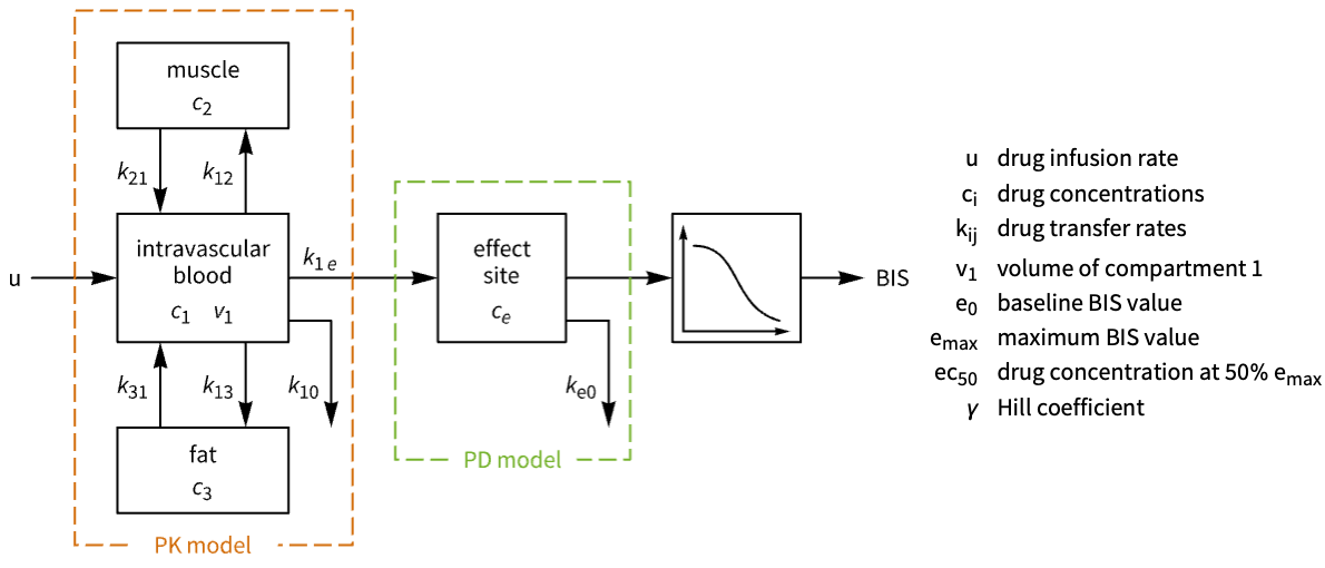
A model of the pharmacokinetic (PK) characteristics:
pk = AffineStateSpaceModel[
 {{(-Subscript[c, 1])*(Subscript[k, 10] + Subscript[k, 12] +
      Subscript[k, 13]) + Subscript[c, 2]*Subscript[k, 21] +
    Subscript[c, 3]*Subscript[k, 31],
   Subscript[c, 1]*Subscript[k, 12] - Subscript[c, 2]*
     Subscript[k, 21], Subscript[c, 1]*Subscript[k, 13] -
    Subscript[c, 3]*Subscript[k, 31]},
  {{Subscript[v, 1]^(-1)}, {0}, {0}}, {Subscript[c, 1]}, {{0}}},
 {Subscript[c, 1], Subscript[c, 2], Subscript[c, 3]},
 {{u, 0}}, {Automatic}, Automatic, SamplingPeriod -> None];
A model of the pharmacodynamic (PD) characteristics:
pd = AffineStateSpaceModel[{{Subscript[c, e]*
    Subscript[k, e0]}, {{-Subscript[k, e]}},
  {Subscript[c, e]}, {{0}}}, {Subscript[c, e]},
 {{Subscript[c, 1], 0}}, {Automatic}, Automatic, SamplingPeriod -> None];
A model of the relationship between the Bispectral Index (BIS) and ![]() using the Hill equation:
using the Hill equation:
hillEq = bis == Subscript[e, 0] - Subscript[e, max]((Subscript[c, e]^γ/Subscript[c, e]^γ + Subscript[ec, 50]^γ)) /. Subscript[e, max] -> Subscript[e, 0] /. {Subscript[e, 0] -> 93.1, Subscript[ec, 50] -> 7.42, γ -> 3}A plot showing the nonlinear characteristics of the Hill equation:
ContourPlot[hillEq, {Subscript[c, e], 0, 25}, {bis, 0, 100}, ContourStyle -> Thick, GridLines -> Automatic, FrameLabel -> {Subscript[c, e], "BIS"}]The compartmental model with ![]() as input and
as input and ![]() as output:
as output:
sys = SystemsModelSeriesConnect[pk, pd] /. IconizedObject[«pars»]A discrete-time approximation of the model:
sysd = ToDiscreteTimeModel[sys, 1]//ChopSet up the cost to track the output:
cost = <|"Horizon" -> 3, "ErrorWeight" -> {{1000}}, "InputIncrementWeight" -> {{1}}|>Compute ![]() for fully awake and moderately but not deeply hypnotic BIS values:
for fully awake and moderately but not deeply hypnotic BIS values:
{Subscript[c, emin], Subscript[c, emax]} = Table[Subscript[c, e] /. NSolve[hillEq, Subscript[c, e], Reals][[1]], {bis, {93.1, 40}}]Specify the constraint to prevent the patient from going into a deep hypnotic state:
cons = Subscript[c, emin] <= Subscript[c, e] <= Subscript[c, emax]cd = ModelPredictiveController[sysd, cost, cons]csys = cd["ClosedLoopSystem"]Compute ![]() to achieve a BIS value of
to achieve a BIS value of ![]() , which puts the patient in a moderate hypnotic state:
, which puts the patient in a moderate hypnotic state:
Subscript[c, eref] = Subscript[c, e] /. NSolve[hillEq /. bis -> 50, Subscript[c, e], Reals][[1]]The ![]() plot of the automated process:
plot of the automated process:
or = OutputResponse[csys, Table[Subscript[c, eref], 100]];
ListStepPlot[%, PlotRange -> All]Show[RegionPlot[{90 ≤ y ≤ 100, 60 ≤ y ≤ 90, 40 ≤ y ≤ 60, 20 ≤ y ≤ 40, y ≤ 20}, {x, 0, 101}, {y, 0, 100}, IconizedObject[«rpOpts»]], ListStepPlot[Table[bis /. NSolve[hillEq, bis, Reals][[1]], {Subscript[c, e], or[[1]]}], IconizedObject[«lpOpts»]], IconizedObject[«sOpts»]]Design a controller to improve an isothermal continuous stirred-tank reactor process: »
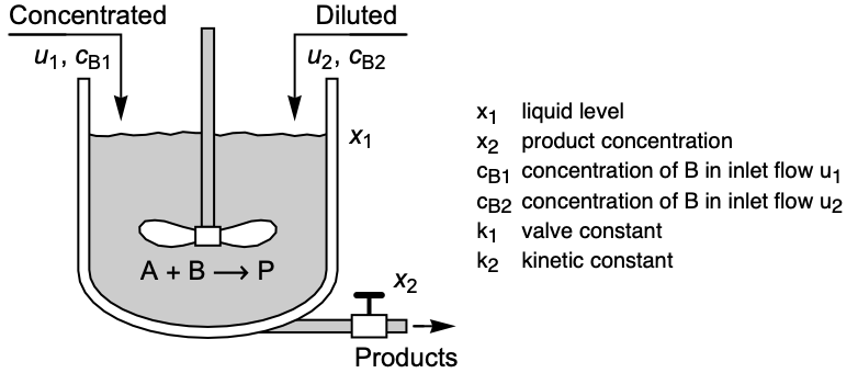
A model of the system with states ![]() and inputs
and inputs ![]() :
:
pars = {Subscript[c, B1] -> 20.05, Subscript[c, B2] -> 0.2, Subscript[k, 1] -> 0.4, Subscript[k, 2] -> 1};cstr = AffineStateSpaceModel[{{(-Subscript[k, 1])*Sqrt[Subscript[x, 1]],
((-Subscript[k, 2])*Subscript[x, 2])/
(1 + Subscript[x, 2])^2},
{{1, 1}, {(Subscript[c, B1] - Subscript[x, 2])/
Subscript[x, 1], (Subscript[c, B2] -
Subscript[x, 2])/Subscript[x, 1]}},
{Subscript[x, 1], Subscript[x, 2]}, {{0, 0}, {0, 0}}},
{{Subscript[x, 1], 25.05}, {Subscript[x, 2], 9}},
{{Subscript[u, 1], 1}, {Subscript[u, 2], 1}}, {Automatic, Automatic},
Automatic, SamplingPeriod -> None] /. pars;Compute a discrete-time approximation of the model:
cstrd = ToDiscreteTimeModel[cstr, 0.1]//SimplifyThe response of the open-loop system:
OutputResponse[{cstrd, {15, 5}}, Table[{1, 1}, 400]];
olp = ListStepPlot[%, PlotStyle -> Dashed]cd = ModelPredictiveController[cstrd, <|"Horizon" -> 3, "StateWeight" -> DiagonalMatrix[{1, 1}], "InputWeight" -> DiagonalMatrix[{1, 1}]|>, {0 <= Subscript[u, 1] <= 5, 0 <= Subscript[u, 2] <= 5}]csys = cd["ClosedLoopSystem"]The response of the closed-loop system:
inp = Table[PadRight[{0}, 400], {2}];or = OutputResponse[{csys, <|1 -> {15, 5}|>}, inp];
clp = ListStepPlot[or]
Compare the open and closed-loop responses:
Show[olp, clp, PlotRange -> All]OutputResponse[cd["ControllerModel"], Join[inp, or]];
ListStepPlot[%, PlotRange -> {{0, 100}, All}]Properties & Relations (3)
LQRegulatorGains is a special case of the squared 2-norm, infinite horizon problem:
LQRegulatorGains[StateSpaceModel[{{{1.5}}, {{1}}, {{1}}, {{0}}}, {x}, {u},
SamplingPeriod -> 1, SystemsModelLabels -> None], {(2), (1)}, "FeedbackGains"]ModelPredictiveController with no constraints gives essentially the same result:
ModelPredictiveController[StateSpaceModel[{{{1.5}}, {{1}}, {{1}}, {{0}}}, {x}, {u},
SamplingPeriod -> 1, SystemsModelLabels -> None],
<|"StateWeight" -> (2), "InputWeight" -> (1), "Norm" -> 2, "Horizon" -> ∞|>, {}, "FeedbackGains"]LQRegulatorGains does not take constraints into consideration:
cdLQR = LQRegulatorGains[StateSpaceModel[{{{1.5}}, {{1}}, {{1}}, {{0}}}, {x}, {u},
SamplingPeriod -> 1, SystemsModelLabels -> None], {(2), (1)}, "Data"]ModelPredictiveController takes state and control constraints into consideration:
cdMPC = ModelPredictiveController[StateSpaceModel[{{{1.5}}, {{1}}, {{1}}, {{0}}}, {x}, {u},
SamplingPeriod -> 1, SystemsModelLabels -> None],
<|"StateWeight" -> (2), "InputWeight" -> (1), "Norm" -> 2, "Horizon" -> ∞|>, {-10 <= x <= 10, -2 <= u <= 2}]Consequently, LQRegulatorGains has only one set of feedback gains:
cdLQR["FeedbackGains"]While the feedback gains of ModelPredictiveController are a piecewise function:
cdMPC["FeedbackGains"]It also computes the region where the feedback is feasible:
Short[cdMPC["FeedbackRegions"]]Compute the bounds of the feasible region:
RegionBounds[%]Simulate the LQR closed-loop system from ![]() , which is outside the feasible region:
, which is outside the feasible region:
orLQR1 = OutputResponse[{cdLQR["ClosedLoopSystem"], {5}}, Table[0, 15]];
ListStepPlot[orLQR1, DataRange -> {0, 15}, PlotRange -> All]
The control constraint ![]() is violated:
is violated:
OutputResponse[cdLQR["ControllerModel"], Join[{Table[0, 15]}, orLQR1]];
ListStepPlot[Join[%, Table[{-2, 2}, 15]], IconizedObject[«plotOpts»]]The closed-loop system's response with the MPC controller from an unfeasible initial value ![]() :
:
orMPC1 = OutputResponse[{cdMPC["ClosedLoopSystem"], <|1 -> {5}|>}, Table[0, 3]]The responses of the LQR and MPC closed-loop systems from a feasible initial value ![]() :
:
orLQR2 = OutputResponse[{cdLQR["ClosedLoopSystem"], {2.8}}, Table[0, 15]];orMPC2 = OutputResponse[{cdMPC["ClosedLoopSystem"], <|1 -> {2.8}|>}, Table[0, 15]];
ListStepPlot[Join[orLQR2, orMPC2], IconizedObject[«plotOpts»]]
The controller response shows that the LQR controller again violates the control constraints:
OutputResponse[cdLQR["ControllerModel"], Join[{Table[0, 15]}, orLQR2]];
OutputResponse[cdMPC["ControllerModel"], Join[{Table[0, 15]}, orMPC2]];
ListStepPlot[Join[%%, %, Table[{-2, 2}, 15]], IconizedObject[«plotOpts»]]An MPC controller is computed by solving multiple multiparametric optimization problems:
a = {{1}};
b = {{1}};
q = {{3}};
r = {{1}};
cons = {-5 <= x <= 5, -1 <= u <= 1};
A function to compute the quadratic cost:
costFn[k_] := Sum[{x[i]}.q.{x[i]} + {u[i]}.r.{u[i]}, {i, k, 2}] + {x[3]}.q.{x[3]}A function to assemble the constraints:
consFn[k_] := Join[Table[Splice[Thread[{x[i + 1]} == a.{x[i]} + b.{u[i]}]], {i, k, 2}], Table[cons[[1]] /. x -> x[i], {i, k, 3}], Table[cons[[2]] /. u -> u[i], {i, k, 2}]]A function to assemble the variables:
varsFn[k_] := Join[Table[u[i], {i, k, 2}], Table[x[i], {i, k + 1, 3}]]Solve the optimization problems for the various instances:
Table[-ArgMin[{costFn[k], consFn[k]}, varsFn[k]][[1]], {k, 0, 2}]//SimplifyModelPredictiveController gives essentially the same result:
ModelPredictiveController[StateSpaceModel[{a, b}, {x}, {u},
	SamplingPeriod -> 1], <|"StateWeight" -> q, "InputWeight" -> r, "Horizon" -> 3|>, cons, "FeedbackGains"]//Simplify
Possible Issues (2)
1- and ![]() -norms with
-norms with ![]() -horizon are not supported:
-horizon are not supported:
ModelPredictiveController[StateSpaceModel[{{{1}}, {{1}}}, SamplingPeriod -> 1, SystemsModelLabels -> None], <|"Norm" -> 1, "Horizon" -> ∞,
	"StateWeight" -> {{10}}, "InputWeight" -> {{1}}|>, {}]
Change it to a squared 2-norm problem:
ModelPredictiveController[StateSpaceModel[{{{1}}, {{1}}}, SamplingPeriod -> 1, SystemsModelLabels -> None], <|"Norm" -> 2, "Horizon" -> ∞,
"StateWeight" -> {{10}}, "InputWeight" -> {{1}}|>, {}]ModelPredictiveController[StateSpaceModel[{{{1}}, {{1}}}, SamplingPeriod -> 1, SystemsModelLabels -> None], <|"Norm" -> 1, "Horizon" -> 4,
"StateWeight" -> {{10}}, "InputWeight" -> {{1}}|>, {}]Constraints for the ![]() horizon problem cannot include
horizon problem cannot include ![]() and
and ![]() terms:
terms:
ModelPredictiveController[StateSpaceModel[{{{-0.3}}, {{1}}, {{1}}, {{0}}}, {x}, {u},
 SamplingPeriod -> 1, SystemsModelLabels -> None], <|"Horizon" -> ∞, "StateWeight" -> {{1}}, "InputWeight" -> {{1}}|>, {-1 <= x[0] <= 1, -1 <= u <= 1}]
Specify constraints using the state and input variables:
ModelPredictiveController[StateSpaceModel[{{{-0.3}}, {{1}}, {{1}}, {{0}}}, {x}, {u},
SamplingPeriod -> 1, SystemsModelLabels -> None], <|"Horizon" -> ∞, "StateWeight" -> {{1}}, "InputWeight" -> {{1}}|>, {-1 <= x <= 1, -1 <= u <= 1}]ModelPredictiveController[StateSpaceModel[{{{-0.3}}, {{1}}, {{1}}, {{0}}}, {x}, {u},
SamplingPeriod -> 1, SystemsModelLabels -> None], <|"Horizon" -> 5, "StateWeight" -> {{1}}, "InputWeight" -> {{1}}|>, {-1 <= x[0] <= 1, -1 <= u <= 1}]Text
Wolfram Research (2022), ModelPredictiveController, Wolfram Language function, https://reference.wolfram.com/language/ref/ModelPredictiveController.html.
CMS
Wolfram Language. 2022. "ModelPredictiveController." Wolfram Language & System Documentation Center. Wolfram Research. https://reference.wolfram.com/language/ref/ModelPredictiveController.html.
APA
Wolfram Language. (2022). ModelPredictiveController. Wolfram Language & System Documentation Center. Retrieved from https://reference.wolfram.com/language/ref/ModelPredictiveController.html