

SpatialEstimate
SpatialEstimate[{loc1val1,loc2val2,…}]
場所 lociで与えられた値 valiからの空間予測を作成する.
SpatialEstimate[{loc1,loc2,…}{val1,val2,…}]
同じ結果を生成する.
詳細とオプション
- SpatialEstimateは,クリギング,地理空間予測,あるいはガウス過程回帰としても知られている.
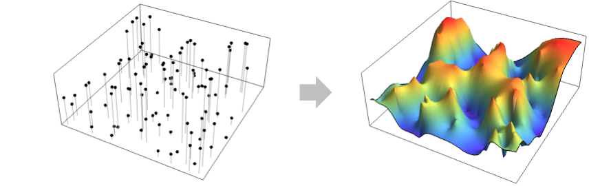
- SpatialEstimateはSpatialEstimatorFunctionを返し,通常は loci以外の場所の値を予測するために使われる.値には,高度,濃度,温度等が含まれる.
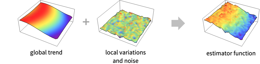
- SpatialEstimateはグローバルトレンドモデルとローカルバリエーションモデルを識別することで作用する.
- ローカルバリエーションの部分は期待される予測誤差
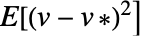 を最小にするために定義される.ただし,
 は真の値で
 は予測された値である.
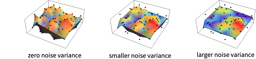
- ローカルバリエーションには2つの部分がある.VariogramFunctionはある場所の値が近くの値にどの程度影響を受けるかを説明し,SpatialNoiseLevelは値の測定値にどの程度のノイズが含まれるかを説明する.
- ノイズの分散が0のとき,予測器関数は指定された値を補間する.ノイズの分散が非零のときは,予測器関数は指定された値を近似するが補間はせず,事実上表面を平坦化する.SpatialNoiseLevelは,事実上,結果のSpatialEstimatorFunctionにおける平坦化レベルの制御法を与える.
- 場所 lociは以下の形でよい.
-
{p1,…,pd} 幾何学的な場所 GeoPosition[…],GeoPositionENU[…],… 地理的な場所 - 値 valiは実数値あるいは数量でよい.
- 次は,使用可能なオプションである.
-
SpatialTrendFunction Automatic グローバルなトレンドモデル VariogramFunction Automatic ローカルなバリエーションモデル SpatialNoiseLevel Automatic valiのノイズレベル
例題
すべて開く すべて閉じる例 (3)
SpatialEstimateは場所とともに与えられる疎な値について連続関数を計算する:
data = {{0.0683671, 0.635233} -> 15.1, {0.110887, 0.823343} -> 25.5, {0.241157, 0.853893} -> 7.9, {0.260237, 1.04258} -> 19.1, {0.266257, 0.964603} -> 19.4, {0.305197, 0.619043} -> 33.4, {0.318197, 0.896843} -> 10.7, {0.376197, 1.15155} -> 29.6, {0.381077, 0.584253} -> 39.4, {0.381277, 0.595373} -> 19.4, {0.537597, 0.804043} -> 12.4, {0.550127, 1.40456} -> 10.5, {0.625677, 1.32567} -> 13.5, {0.636097, 0.758103} -> 28.5, {0.635167, 0.135353} -> 11.4, {0.717057, 1.12401} -> 33.4, {0.785927, 0.511553} -> 13.1, {0.834457, 0.0217334} -> 7.8, {0.846227, 1.14474} -> 29.8, {1.00857, 0.565023} -> 14.1};PointValuePlot[data]sef = SpatialEstimate[data]sef[{.2, .4}]Plot3D[sef[{x, y}], {x, 0, 1}, {y, 0, 1.5}]locs = {...};
vals = {...};PointValuePlot[locs -> vals]sef = SpatialEstimate[locs -> vals, SpatialTrendFunction -> 0]DensityPlot[sef[{x, y}], {x, y}∈RipleyRassonRegion[locs]]data = SpatialPointData[«2»];Show[Region[data["ObservationRegion"]], PointValuePlot[data, ColorFunction -> "Rainbow"]]spf = SpatialEstimate[data -> "Rainfall", SpatialTrendFunction -> 1]pts = RandomPoint[data["ObservationRegion"], 3000];PointValuePlot[pts -> spf[pts], ColorFunction -> "Rainbow", FrameTicks -> None, AspectRatio -> 2 / 3]スコープ (2)
m = 25;
data = RandomReal[1, {m, 2}] -> RandomReal[1, m];varfn = VariogramModel["Exponential", {1, 1}, SpatialNoiseLevel -> 0.1]空間推定器関数をバリオグラムモデルと二次トレンドで作成する:
spf = SpatialEstimate[data, VariogramFunction -> varfn, SpatialTrendFunction -> 2]spf["Visualization", "Data" -> True]SpatialEstimateを指定のバリオグラム関数と一緒に使う:
locs = {...};
vals = {...};PointValuePlot[locs -> vals]sef = SpatialEstimate[locs -> vals, SpatialTrendFunction -> 1]sef[ "VariogramModelName"]vf = EstimatedVariogramModel[locs -> vals, "Exponential"]vf["Visualization"]sef2 = SpatialEstimate[locs -> vals, VariogramFunction -> vf, SpatialTrendFunction -> 1]{sef["Visualization"], sef2["Visualization"]}オプション (4)
SpatialNoiseLevel (1)
SpatialNoiseLevelを使ってノイズレベルを指定する:
m = 30;
{datapoints, datavalues} = RandomReal[1, {2, m}];
data = datapoints -> datavalues;spf = SpatialEstimate[data, SpatialNoiseLevel -> .1]spf["Visualization"]ノイズレベルが0ならSpatialEstimateは厳密に補間する:
spf = SpatialEstimate[data, SpatialNoiseLevel -> 0]spf["Visualization"]SpatialTrendFunction (1)
SpatialTrendFunctionを使ってトレンド関数を指定する:
m = 25;
data = RandomReal[1, {m, 2}] -> RandomReal[1, m];PointValuePlot[data, ColorFunction -> "Rainbow"]spf0 = SpatialEstimate[data, SpatialTrendFunction -> 0]spf0["Visualization"]spf2 = SpatialEstimate[data, SpatialTrendFunction -> 2]spf2["Visualization"]VariogramFunction (1)
VariogramFunctionを使ってバリオグラムモデルを指定する:
m = 100;
SeedRandom[1];
{datapoints, datavalues} = RandomReal[1, {2, m}];
data = datapoints -> datavalues;spf = SpatialEstimate[data, VariogramFunction -> "Exponential"]spf["Visualization", AxesOrigin -> {0, 0}]フィット済みのVariogramModelを使う:
var = EstimatedVariogramModel[data, "Gaussian"]SpatialEstimate[data, VariogramFunction -> var]%["Visualization", AxesOrigin -> {0, 0}]DistanceFunction (1)
DistanceFunctionを使って距離関数を指定する:
m = 100;
data = RandomReal[1, {m, 2}] -> RandomReal[1, m];spf = SpatialEstimate[data, DistanceFunction -> (Norm[Subtract[#1, #2], 8]&)]spf["Visualization"]アプリケーション (4)
空間データは,例えば衛星のオゾン測定値のように,しばしば領域が欠落している規則的な格子で与えられる:
locs = GeoPosition[{{25.5, -124.5}, {25.5, -123.5}, {25.5, -122.5}, {25.5, -121.5}, {25.5, -120.5},
{25.5, -112.5}, {25.5, -111.5}, {25.5, -110.5}, {25.5, -109.5}, {25.5, -108.5}, {25.5, -107.5},
{25.5, -106.5}, {25.5, -105.5}, {25.5, -104.5}, {25.5 ... 8.5, -87.5}, {48.5, -86.5},
{48.5, -85.5}, {48.5, -84.5}, {48.5, -83.5}, {48.5, -82.5}, {48.5, -81.5}, {48.5, -80.5},
{48.5, -79.5}, {48.5, -78.5}, {48.5, -72.5}, {48.5, -71.5}, {48.5, -70.5}, {48.5, -69.5},
{48.5, -68.5}, {48.5, -67.5}}];ozone = {...};PointValuePlot[locs -> ozone, ColorFunction -> "Rainbow"]sf = SpatialEstimate[locs -> ozone]sf[Entity["City", {"Boston", "Massachusetts", "UnitedStates"}]]観測領域内の一様のランダムな場所で空間推定器関数を評価する:
reg = Entity["Country", "UnitedStates"]["Polygon"];pts = RandomGeoPosition[reg, 3000]PointValuePlot[pts -> sf[pts], ColorFunction -> "Rainbow"]SpatialEstimateを使って疎な観測場所から連続推定を作成する:
data = ResourceData["Sample Data: Swiss Rainfall"]Show[Region[data["ObservationRegion"]], PointValuePlot[data, ColorFunction -> "Rainbow"]]models = {"Cubic", "Spherical", "Exponential", "Gaussian"};estimates = SpatialEstimate[data, VariogramFunction -> #]& /@ models;ランダムな点の集合を作成し,それらの場所における推定値を計算する:
pts = RandomPoint[data["ObservationRegion"], 2000];
vals = Through[estimates[pts]];Grid@ArrayReshape[#, {2, 2}]&@MapThread[Show[Region[data["ObservationRegion"]], PointValuePlot[pts -> #1, PlotStyle -> PointSize[0.015], ColorFunction -> "Rainbow"], PlotLabel -> #2]&, {vals, models}]SpatialEstimateはデータのより滑らかな画像が作成できる:
locs = {...};
vals = {...};{PointValuePlot[locs -> vals, ColorFunction -> "Rainbow"], ListDensityPlot[ArrayFlatten[{{locs, Partition[vals, 1]}}], ColorFunction -> "Rainbow"]}est0 = SpatialEstimate[locs -> vals, SpatialNoiseLevel -> .0001];
est1 = SpatialEstimate[locs -> vals, SpatialNoiseLevel -> .1];reg = Rectangle[{0, 0}, {Max[locs[[All, 1]]], Max[locs[[All, 2]]]}];pts = RandomPoint[reg, 5 * 10 ^ 3];
res0 = est0[pts];
res1 = est1[pts];MapThread[PointValuePlot[pts -> #1, PlotStyle -> PointSize[.02], ColorFunction -> "Rainbow", PlotLabel -> #2]&, {{res0, res1}, {"smaller noise level", "larger noise level"}}]{Mean@est0[pts, Around], Mean@est1[pts, Around]}RegionMeasure[reg]大西洋におけるホタテのサンプルの場所.捕獲されたサンプルの総数と補充前および成体の数が注釈として付けられている:
obj = ResourceObject["Sample Data: Scallop Abundance"]obj["Description"]data = ResourceData[obj]pos = Position[data["Annotations"]["Catch"], _ ? Positive];
locs = Extract[data["Points"], pos];recruitsRate = Extract[data["Annotations"]["Recruits"], pos] / Extract[data["Annotations"]["Catch"], pos]//N;SpatialEstimateを使って捕獲率が低い場所の補充率を作成する:
est = SpatialEstimate[locs -> recruitsRate, VariogramFunction -> "Gaussian"]ランダムな点集合を作成し,それらの場所における推定値を計算する:
pts = RandomPoint[data["ObservationRegion"], 3000];
vals = est[pts];Row@{PointValuePlot[locs -> recruitsRate, ColorFunction -> "Rainbow", PlotLegends -> Automatic, PlotLabel -> "recruits rates"], PointValuePlot[pts -> vals, PlotStyle -> PointSize[Small], ColorFunction -> "Rainbow", PlotLabel -> "estimated recruits rates"]}特性と関係 (2)
大きい空間ノイズレベルについて,空間推定器はトレンド関数に収束する:
locs = Range[0, 1, 0.05];
vals = {...};dataPlot = ListPlot[Transpose[{locs, vals}], PlotStyle -> Green]指定された多項式トレンド次数について,増大するノイズレベルの値についてのSpatialEstimateを計算する:
trend = {1, 2, 3};
noise = {0, 0.01, .05, 5};
est = Table[SpatialEstimate[locs -> vals, SpatialTrendFunction -> tr, SpatialNoiseLevel -> ns]//Quiet, {ns, noise}, {tr, trend}];plots = Table[Show[dataPlot,
Plot[{est[[k, 1]][x], est[[k, 2]][x], est[[k, 3]][x]}, {x, 0, 1}], PlotLabel -> Row[{"noise level = ", noise[[k]]}]], {k, 1, 4}];
legend = LineLegend[{RGBColor[0.368417, 0.506779, 0.709798], RGBColor[0.880722, 0.611041, 0.142051], RGBColor[0.560181, 0.691569, 0.194885]}, {"linear", "square", "cubic"}, LegendLabel -> "trend"];
Legended[Grid[ArrayReshape[plots, {2, 2}]], legend]SpatialNoiseLevelがゼロのときにのみSpatialEstimateは厳密な補間器になる:
locs = Range[0, 1, 0.05];
vals = {...};dataPlot = ListPlot[Transpose[{locs, vals}], PlotStyle -> Green]est0 = SpatialEstimate[locs -> vals, SpatialNoiseLevel -> 0];estSmall = SpatialEstimate[locs -> vals, SpatialNoiseLevel -> 0.005];estLarge = SpatialEstimate[locs -> vals, SpatialNoiseLevel -> 0.05];Show[dataPlot, Plot[{est0[x], estSmall[x], estLarge[x]}, {x, 0, 1}, PlotLegends -> {"zero noise level", "smaller noise level", "larger noise level"}]]考えられる問題 (1)
SeedRandom["bad"];
{locs, vals} = RandomReal[1, {2, 10}];
data = locs -> vals;var0 = VariogramModel["Gaussian", {1, 10}, SpatialNoiseLevel -> 0];
sef0 = SpatialEstimate[locs -> vals, VariogramFunction -> var0];sef0["Visualization"]正のSpatialNoiseLevelを許容すると正規化として機能する:
var1 = VariogramModel["Gaussian", {1, 10}];
sef1 = SpatialEstimate[locs -> vals, VariogramFunction -> var1];sef1[SpatialNoiseLevel]sef1["Visualization"]おもしろい例題 (1)
locs = GeoPosition@EntityValue[EntityClass["Country", "Europe"], "Position"]pops = EntityValue[EntityClass["Country", "Europe"], "Population"];PointValuePlot[locs -> pops, ColorFunction -> "Rainbow"]指数バリオグラムモデルと異なる2つのトレンドモデルで推定器曲面を求める:
spfConstTrend = SpatialEstimate[locs -> pops, VariogramFunction -> "Exponential", SpatialTrendFunction -> 0]spfLinearTrend = SpatialEstimate[locs -> pops, VariogramFunction -> "Exponential", SpatialTrendFunction -> 2]samples = RandomGeoPosition[Entity["GeographicRegion", "Europe"]["Polygon"], 600]PointValuePlot[samples -> #[samples], ColorFunction -> "Rainbow"]& /@ {spfConstTrend, spfLinearTrend}テキスト
Wolfram Research (2021), SpatialEstimate, Wolfram言語関数, https://reference.wolfram.com/language/ref/SpatialEstimate.html.
CMS
Wolfram Language. 2021. "SpatialEstimate." Wolfram Language & System Documentation Center. Wolfram Research. https://reference.wolfram.com/language/ref/SpatialEstimate.html.
APA
Wolfram Language. (2021). SpatialEstimate. Wolfram Language & System Documentation Center. Retrieved from https://reference.wolfram.com/language/ref/SpatialEstimate.html