LinearModelFit

LinearModelFit[{{x₁,y₁},{x₂,y₂},…},{f₁,f₂,…},x]

constructs a linear model of the form that fits the y_i for successive x_i values.

LinearModelFit[data,{f₁,f₂,…},{x₁,x₂,…}]

constructs a linear model where the f_i depend on the variables x_k.

LinearModelFit[{m,v}]

constructs a linear model from the design matrix m and response vector v.

Details and Options

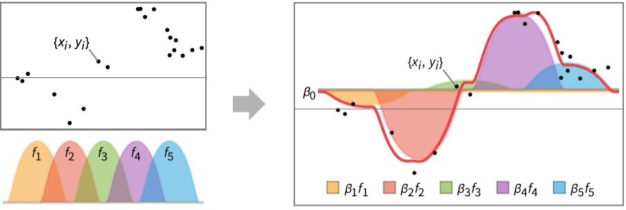
LinearModelFit attempts to model the input data using a linear combination of functions.
LinearModelFit produces a linear model of the form under the assumption that the original are independent normally distributed with mean and common standard deviation.

LinearModelFit returns a symbolic FittedModel object to represent the linear model it constructs.
The value of the best-fit function from LinearModelFit at a particular point x₁, … can be found from model[x₁,…].
Possible forms of data are:

	{y₁,y₂,…}	equivalent to the form {{1,y₁},{2,y₂},…}
	{{x₁₁,x₁₂,…,y₁},…}	a list of independent values x_ij and the responses y_i
	{{x₁₁,x₁₂,…}y₁,…}	a list of rules between input values and response
	{{x₁₁,x₁₂,…},…}{y₁,y₂,…}	a rule between a list of input values and responses
	{{x₁₁,…,y₁,…},…}n	fit the n column of a matrix
	Tabular[…]name	fit the column name in a tabular object

With multivariate data such as ${{x_(11),x_(12),... ,y_(1)},{x_(21),x_(22),... ,y_(2)},...}$ , the number of coordinates x_i1, x_i2, … should equal the number of variables x_i.
The data points can be approximate real numbers. Uncertainty can be specified using Around.
Additionally, data can be specified using a design matrix without specifying functions and variables:
{m,v} a design matrix m and response vector v
In LinearModelFit[{m,v }], the design matrix m is formed from the values of basis functions f_i at data points in the form {{f₁,f₂,…},{f₁,f₂,…},…}. The response vector v is the list of responses {y₁,y₂,…}.
When a design matrix is used, the basis functions f_i can be specified using the form LinearModelFit[{m,v},{f₁,f₂,…}].
For a design matrix m and response vector v, the model is , where is the vector of parameters to be estimated.

Options

LinearModelFit takes the following options:

ConfidenceLevel	95/100	confidence level to use for parameters and predictions
IncludeConstantBasis	True	whether to include a constant basis function
LinearOffsetFunction	None	known offset in the linear predictor
NominalVariables	None	variables considered as nominal or categorical
VarianceEstimatorFunction	Automatic	function for estimating the error variance
Weights	Automatic	weights for data elements
WorkingPrecision	Automatic	precision used in internal computations

With the setting IncludeConstantBasis->False, a model of the form is fitted. The option IncludeConstantBasis is ignored if the design matrix is specified in the input.
With the setting LinearOffsetFunction->h, a model of the form is fitted.
With ConfidenceLevel->p, probability-p confidence intervals are computed for parameter and prediction intervals.
With the setting Weights->{w₁,w₂,…}, the error variance for y_i is assumed proportional to .
With the setting Weights->Automatic, the weights will be set to 1 if the data contains exact values. If the data contains Around values, the weights will be set to with the total response variance.
The total response variance is a function of the initial response variance s_i² and the independent values variance .
The are propagated through the model using AroundReplace and the resulting variance is added to response variance s_i². The function FindRoot is used internally to find a self-consistent solution according to the Fasano and Vio method.
With the setting VarianceEstimatorFunction->f, the variance is estimated by f[res,w], where res={y₁-,y₂-,…} is the list of residuals and w={w₁,w₂,…} is the list of weights for the measurements y_i.
Using VarianceEstimatorFunction->(1&) and Weights->{1/Δy₁²,1/Δy₂²,…}, Δy_i is treated as the known uncertainty of measurement y_i, and parameter standard errors are effectively computed only from the weights.

Properties

The properties and diagnostics of the FittedModel can be obtained from model["property"].
Properties related to data and the fitted function obtained using model["property"] include:

	"BasisFunctions"	list of basis functions
	"BestFit"	fitted function
	"BestFitParameters"	parameter estimates
	"Data"	the input data or design matrix and response vector
	"DesignMatrix"	design matrix for the model
	"Function"	best fit pure function
	"Response"	response values in the input data
	"Weights"	weights used to fit the data

Types of residuals include:

	"FitResiduals"	difference between actual and predicted responses
	"StandardizedResiduals"	fit residuals divided by the standard error for each residual
	"StudentizedResiduals"	fit residuals divided by single deletion error estimates

Properties related to the sum of squared errors include:

	"ANOVA"	analysis of variance data
	"CoefficientOfVariation"	estimated standard deviation divided by the response mean
	"EstimatedVariance"	estimate of the error variance
	"PartialSumOfSquares"	changes in model sum of squares as nonconstant basis functions are removed
	"SequentialSumOfSquares"	the model sum of squares partitioned componentwise

Properties and diagnostics for parameter estimates include:

	"CorrelationMatrix"	parameter correlation matrix
	"CovarianceMatrix"	parameter covariance matrix
	"Eigenstructure"	eigenstructure of the parameter correlation matrix
	"ParameterEstimates"	table of fitted parameter information
	"VarianceInflationFactors"	list of inflation factors for the estimated parameters

Properties related to influence measures include:

	"BetaDifferences"	DFBETAS measures of influence on parameter values
	"CatcherMatrix"	catcher matrix
	"CookDistances"	list of Cook distances
	"CovarianceRatios"	COVRATIO measures of observation influence
	"DurbinWatsonD"	Durbin–Watson ‐statistic for autocorrelation
	"FitDifferences"	DFFITS measures of influence on predicted values
	"FVarianceRatios"	FVARATIO measures of observation influence
	"HatDiagonal"	diagonal elements of the hat matrix
	"SingleDeletionVariances"	list of variance estimates with the data point omitted

Properties of predicted values include:

	"MeanPredictionBands"	confidence bands for mean predictions
	"MeanPredictions"	confidence intervals for the mean predictions
	"PredictedResponse"	fitted values for the data
	"SinglePredictionBands"	confidence bands based on single observations
	"SinglePredictions"	confidence intervals for the predicted response of single observations

Properties that measure goodness of fit include:

	"AdjustedRSquared"	adjusted for the number of model parameters
	"AIC"	Akaike Information Criterion
	"AICc"	finite sample corrected AIC
	"BIC"	Bayesian Information Criterion
	"RSquared"	coefficient of determination

For the properties "RSquared" and "AdjustedRSquared", the computation of the total sum of squares is mean adjusted only when the constant basis is included.
"PredictedResponse" fitted values for the data

"SinglePredictionBands" confidence bands based on single observations

Examples

open allclose all

Basic Examples (1)

Fit a linear model to some data:

Obtain the functional form:

Evaluate the model at a point:

Visualize the fitted function with the data:

Extract information about the fitting:

Plot the residuals:

Scope (18)

Data (8)

Fit a model of one variable assuming increasing integer independent values:

This is equivalent to:

Fit a model of more than one variable, assuming the response is the last one:

This is equivalent to:

Specify a column as the response:

Fit a list of rules:

Fit a rule of input values and responses:

Fit a model with categorical predictor variables:

Fit a model given a design matrix and response vector:

Fit the model referring to the basis functions as x and y:

Fit a Tabular object by specifying the response column:

Model (3)

Find the best fit linear coefficient for a function:

Fit data to a linear combination of linear functions of independent variables:

This is equivalent to explicitly specifying a constant function:

Fit data to a linear combination of nonlinear functions of independent variables:

Properties (7)

Data & Fitted Functions (1)

Fit a linear model:

Obtain a list of available properties for a linear model:

Extract the original data:

Obtain and plot the best fit:

Obtain the fitted function as a pure function:

Get the design matrix and response vector for the fitting:

Residuals (1)

Examine residuals for a fit:

Visualize the raw fit residuals:

Visualize scaled residuals in stem plots:

Plot the absolute differences between the standardized and Studentized residuals:

Sums of Squares (1)

Fit a linear model to some data:

Extract the estimated error variance and coefficient of variation:

Obtain an analysis of variance table for the model:

Get the F-statistics from the table:

Parameter Estimation Diagnostics (1)

Obtain a formatted table of parameter information:

Obtain the -statistics of fitted parameters:

Influence Measures (1)

Fit some data containing extreme values to a linear model:

Use single deletion variances to check the impact on the error variance of removing each point:

Check Cook distances to identify highly influential points:

Use DFFITS values to assess the influence of each point on the fitted values:

Use DFBETAS values to assess the influence of each point on each estimated parameter:

Prediction Values (1)

Fit a linear model:

Plot the predicted values against the observed values:

Obtain tabular results for the mean prediction confidence intervals:

Obtain tabular results for the single prediction confidence intervals:

Get the single prediction intervals from the table:

Extract 99% mean prediction bands:

Goodness-of-Fit Measures (1)

Obtain a table of goodness-of-fit measures for a linear model:

Compute goodness-of-fit measures for all possible linear submodels:

Rank the models by :

Rank the models by adjusted , which penalizes for adding terms:

Generalizations & Extensions (1)

Perform other mathematical operations on the functional form of the model:

Integrate symbolically and numerically:

Find a predictor value that gives a particular value for the model:

Options (11)

ConfidenceLevel (1)

The default gives 95% confidence intervals:

Use 99% intervals instead:

Set the level to 90% within FittedModel:

IncludeConstantBasis (1)

Fit a simple linear regression model:

Fit the linear model with intercept zero:

LinearOffsetFunction (1)

Fit data to a linear model:

Fit data to a linear model with a known Sqrt[x] term:

NominalVariables (1)

Fit data treating the first variable as a nominal variable:

Treat both variables as nominal:

VarianceEstimatorFunction (1)

Use the default unbiased estimate of error variance:

Assume a known error variance:

Estimate the variance by the mean squared error:

Weights (5)

Fit a model using equal weights:

Give explicit weights for the data points:

Use Around values to give different weights to data points:

Find the weights that were used to account for the uncertainty in the data:

Use Around values in both the independent values and responses:

Fit a model of more than one variable with Around values:

Try the FixedPoint algorithm to find the weights for the model:

Reduce the DampingFactor and increase the MaxIterations to reach convergence:

WorkingPrecision (1)

Use WorkingPrecision to get higher precision in parameter estimates:

Obtain the fitted function:

Reduce the precision in property computations after the fitting:

Applications (6)

Fit the first 100 primes to a linear model:

Visualize the fit:

The systematic trend in the residuals violates the assumption of independent normal errors:

Fit a linear model of multiple variables:

Visually inspect the residuals by data point:

Plot the residuals against each predictor variable:

Plot Cook's distances to diagnose leverage:

Find the positions of distances above a given cutoff value:

Extract the associated data points:

Use - plots to check the assumption of normal errors:

Compare standardized residuals to standard normal values:

Do the comparison with Studentized residuals:

Simulate some data with a continuous and a nominal variable:

Fit an analysis of covariance model to the data:

Obtain an analysis of variance table for the model:

Group the data by treatment:

Visualize the grouped data and associated curves:

Use properties to compute additional results:

Extract the design matrix and residuals:

Compute White's heteroskedasticity-consistent covariance estimate:

Compare with the covariance assuming homoskedasticity:

Compare standard errors based on the two covariance estimates:

Perform a Breusch–Pagan test:

Fit a model:

Fit the squared errors to a model with the same predictors:

Compute the Breusch–Pagan test statistic:

Compute the -value:

Properties & Relations (9)

DesignMatrix constructs the design matrix used by LinearModelFit:

By default, LinearModelFit and GeneralizedLinearModelFit fit equivalent models:

LinearModelFit fits linear models assuming normally distributed errors:

NonlinearModelFit fits nonlinear models assuming normally distributed errors:

Fit and LinearModelFit fit equivalent models:

LinearModelFit allows for extraction of additional information about the fitting:

Fit a linear model to data:

Perform the same fitting using a design matrix and response vector:

Obtain the parameter estimates via LeastSquares:

LinearModelFit fits linear models:

FindFit gives parameter estimates for linear and nonlinear models:

LinearModelFit will use the time stamps of a TimeSeries as variables:

Rescale the time stamps and fit again:

Find fit for the values:

LinearModelFit acts pathwise on a multipath TemporalData:

Do a simple linear model fit:

Do the same fit using a neural net with a single linear layer:

Top