Introduction to Graph Drawing
| Graph Theory Notations | Selecting the Appropriate Graph Drawing Function |
| Input Formats | References |
| Graph Drawing Algorithms |
| GraphPlot | generate a plot of a graph |
| GraphPlot3D | generate a 3D plot of a graph |
| LayeredGraphPlot | generate a layered plot of a graph |
| TreePlot | generate a tree plot of a graph |
{Map[#[{4 -> 2, 4 -> 3, 5 -> 2, 5 -> 3, 5 -> 4, 6 -> 2, 6 -> 3, 6 -> 4, 6 -> 5, 6 -> 7, 7 -> 8, 7 -> 9}, PlotRangePadding -> Automatic, ImageSize -> 180, PlotLabel -> #]&, {{GraphPlot, GraphPlot3D}, {LayeredGraphPlot, TreePlot}}, {-1}]}//TableFormGraphPlot[{4 -> 3, 5 -> 3, 5 -> 4, 6 -> 1, 6 -> 2, 6 -> 4, 6 -> 5}, DirectedEdges -> True]GraphPlot[{4 -> 3, 5 -> 3, 5 -> 4, 6 -> 1, 6 -> 2, 6 -> 4, 6 -> 5}]GraphPlot[{1 -> 2, 2 -> 3, 3 -> 1, 3 -> 4}, DirectedEdges -> True,
VertexLabels -> Automatic]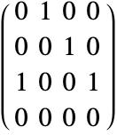
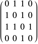
GraphPlot[(|   |   |   |   |
| - | - | - | - |
| 0 | 1 | 1 | 0 |
| 1 | 0 | 1 | 0 |
| 1 | 1 | 0 | 1 |
| 0 | 0 | 1 | 0 |), VertexLabels -> Automatic]SparseArray[{{1, 2} -> 1, {1, 3} -> 1, {2, 1} -> 1, {2, 3} -> 1, {3, 1} -> 1, {3, 2} -> 1, {3, 4} -> 1, {4, 3} -> 1}, {4, 4}];Spring Embedding
GraphPlot[GridGraph[{20, 20}], GraphLayout -> "SpringEmbedding"]Spring-Electrical Embedding
GraphPlot[GridGraph[{20, 20}], GraphLayout -> "SpringElectricalEmbedding"]High-Dimensional Embedding Algorithm
GraphPlot[GridGraph[{20, 20}], GraphLayout -> "HighDimensionalEmbedding"]A Hierarchical Drawing Algorithm for Directed Graphs
1. Vertices of the DAG are first assigned a preliminary ![]() ranking such that if there is an edge from
ranking such that if there is an edge from ![]() to
to ![]() , then it is likely that
, then it is likely that ![]() . This is to ensure that the final drawing has directed edges pointing mostly downward.
. This is to ensure that the final drawing has directed edges pointing mostly downward.
2. The ![]() coordinates are generated so that if there is an edge from
coordinates are generated so that if there is an edge from ![]() to
to ![]() and
and ![]() , their
, their ![]() coordinates are as close as possible, but separated by a set minimum. This ensures that the final resulting drawing does not have many long edges. This process assigns the vertices into a finite number of layers. If an edge lies across a number of layers, virtual vertices are added.
coordinates are as close as possible, but separated by a set minimum. This ensures that the final resulting drawing does not have many long edges. This process assigns the vertices into a finite number of layers. If an edge lies across a number of layers, virtual vertices are added.
3. A preliminary ![]() ranking is assigned to each vertex to minimize the number of edge crossings.
ranking is assigned to each vertex to minimize the number of edge crossings.
4. The ![]() coordinates are generated by minimizing
coordinates are generated by minimizing ![]() subject to the constraints that vertices on the same layer obey the
subject to the constraints that vertices on the same layer obey the ![]() ranking generated in step 3 and are separated by a set minimum.
ranking generated in step 3 and are separated by a set minimum.
Algorithms for Drawing Trees
[1] Di Battista, G., P. Eades, R. Tamassia, and I. G. Tollis. Graph Drawing: Algorithms for the Visualization of Graphs. Prentice Hall, 1999.
[2] Fruchterman, T. M. J. and E. M. Reingold. "Graph Drawing by Force-Directed Placement." Software—Practice and Experience 21, no. 11 (1991): 1129–1164.
[3] Eades, P. "A Heuristic for Graph Drawing." Congressus Numerantium 42 (1984): 149–160.
[4] Quinn, N. and M. Breuer. "A Force Directed Component Placement Procedure for Printed Circuit Boards." IEEE Trans. on Circuits and Systems 26, no. 6 (1979): 377–388.
[5] Kamada, T. and S. Kawai. "An Algorithm for Drawing General Undirected Graphs." Information Processing Letters 31 (1989): 7–15.
[6] Harel, D. and Y. Koren. "Graph Drawing by High-Dimensional Embedding." In Proceedings of 10th Int. Symp. Graph Drawing (GD'02), 207–219, 2002.
[7] Walshaw, C. "A Multilevel Algorithm for Force-Directed Graph-Drawing." J. Graph Algorithms Appl. 7, no. 3 (2003): 253–285.
[8] Cuthill, E. and J. McKee. "Reducing the Bandwidth of Sparse Symmetric Matrices." In Proceedings, 24th National Conference of ACM, 157–172, 1969.
[9] Lim, A., B. Rodrigues, and F. Xiao. "A Centroid-Based Approach to Solve the Bandwidth Minimization Problem." In Proceedings of the 37th Annual Hawaii International Conference on System Sciences (HICSS'04), 30075.1, 2004.
[10] Barnard, S. T., A. Pothen, and H. D. Simon. "A Spectral Algorithm for Envelope Reduction of Sparse Matrices." Journal of Numerical Linear Algebra with Applications 2, no. 4 (1995): 317–334.
[11] Sloan, S. "A Fortran Program for Profile and Wavefront Reduction." International Journal for Numerical Methods in Engineering 28, no. 11 (1989): 2651–2679.
[12] Reid, J. K. and J. A. Scott. "Ordering Symmetric Sparse Matrices for Small Profile and Wavefront." International Journal for Numerical Methods in Engineering 45, no. 12 (1999): 1737–1755.
[13] George, J. A. "Computer Implementation of the Finite-Element Method." Report STAN CS-71-208, PhD Thesis, Department of Computer Science, Stanford University, Stanford, California, 1971.
[14] Sugiyama, K., S. Tagawa, and M. Toda. "Methods for Visual Understanding of Hierarchical Systems." IEEE Trans. Syst. Man, Cybern. 11, no. 2 (1981): 109–125.
[15] Gansner, E. R., E. Koutsofios, S. C. North, and K. P. Vo. "A Technique for Drawing Directed Graphs." IEEE Trans. Software Engineering 19, no. 3 (1993): 214–230.
[16] Quigley, A. "Large Scale Relational Information Visualization, Clustering, and Abstraction." PhD Thesis, Department of Computer Science and Software Engineering, University of Newcastle, Australia, 2001.
[17] Hu, Y. F. "Efficient, High-Quality Force-Directed Graph Drawing." The Mathematica Journal 10, no. 1 (2006): 37–71.