Acoustic Cloak
| Introduction | Model without Acoustic Cloak |
| Pressure Acoustics Model | Model with Acoustic Cloak |
| Domain | Nomenclature |
| Mesh Generation | Reference |
| Boundary Conditions |
Introduction
Acoustic waves can be used to navigate, communicate with or detect objects on or under the surface of water. For example, the sonar system locates an object by emitting pulses of sounds and listening for echoes. However, recent studies [1] have shown the feasibility of hiding an object from sound radiation and making it transparent to the detection system. The concept is to wrap the hidden object with an "acoustic cloak", which is made of multilayered composite materials.
The following model simulates a right-going acoustic wave incident on a hard-walled cylinder. The simulation will be performed with and without the cloak. The resulting sound-scattering patterns will then be compared to quantify the effectiveness of the acoustic cloak.
The symbols and corresponding units used throughout this tutorial are summarized in the Nomenclature section.
Please refer to the information provided in "Acoustics in the Frequency Domain" for more general theoretical background on acoustics.
Needs["NDSolve`FEM`"]Pressure Acoustics Model
To describe the propagation of harmonic sound waves, the Helmholtz partial differential equation (PDE) is used. Since an infinitely extended domain is needed, the Helmholtz equation is transformed with a perfectly matched layer (PML). The derivation and the theoretical background of the perfectly matched layer (PML) can be found in the acoustics frequency domain tutorial. The transformation of the Helmholtz equation with the perfectly matched layer results in the following equation:
Here, ![]() and
and ![]() are the absorbing coefficients of the PML, and two auxiliary parameters,
are the absorbing coefficients of the PML, and two auxiliary parameters, ![]() and
and ![]() , are introduced to control the PML attenuation in each dimension.
, are introduced to control the PML attenuation in each dimension.
vars = {p[x, y], ω, {x, y}};
FrequencyPMLModel = DiffusionPDETerm[vars, 1 / (ρ{sx / sy, sy / sx})] - ReactionPDETerm[vars, (sx sy ω^2/ρ c^2)]getPMLparameters[var_, pmlBoundary_, pmlWidth_, σMax_, c_, ω_] := Module[{σ},
With[{p1 = pmlBoundary[[1]], p2 = pmlBoundary[[2]]},
σ = Simplify[Which[
var - p1 ≥ 0, ((var - p1) / pmlWidth)^2 * σMax,
p2 - var ≥ 0, ((p2 - var) / pmlWidth)^2 * σMax,
True, 0], TimeConstraint -> 1]];
1 - I c σ / ω]Domain
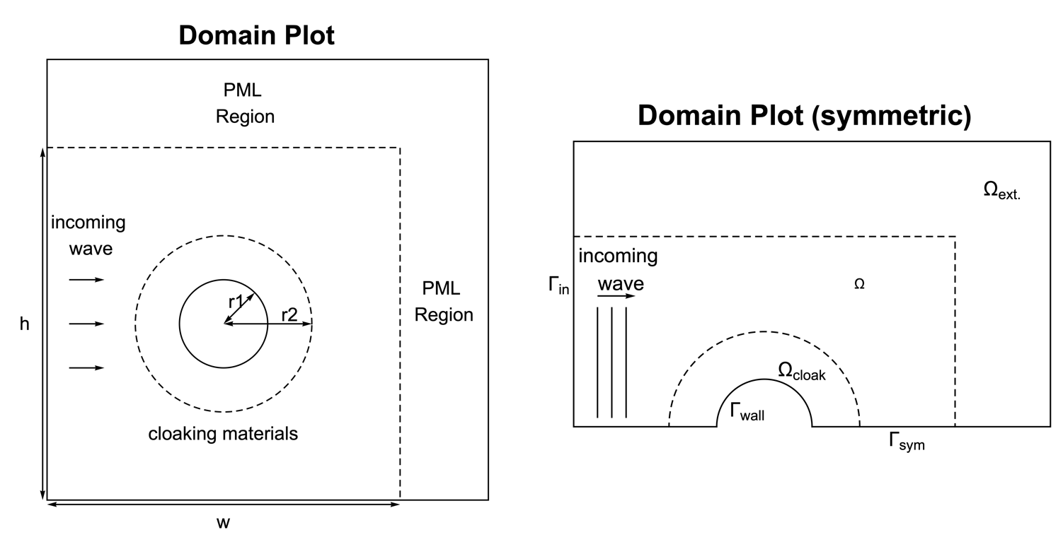
In the geometric model, a rigid cylinder with the radius ![]() is surrounded by layers of acoustic cloaking materials up until an outer radius
is surrounded by layers of acoustic cloaking materials up until an outer radius ![]() . A time-harmonic sound wave is set to enter the domain from the left as a probe signal. To build an infinitely extended domain in both the
. A time-harmonic sound wave is set to enter the domain from the left as a probe signal. To build an infinitely extended domain in both the ![]() and
and ![]() directions, the computational domain is extended to include a PML region, which absorbs the outgoing/scattering wave.
directions, the computational domain is extended to include a PML region, which absorbs the outgoing/scattering wave.
Due to the symmetry along the ![]() axis of the geometry, it is efficient to construct the simulation domain
axis of the geometry, it is efficient to construct the simulation domain ![]() with only the upper half of the cylinder. The cylinder wall boundary and the symmetric boundary are symbolized as
with only the upper half of the cylinder. The cylinder wall boundary and the symmetric boundary are symbolized as ![]() and
and ![]() , respectively.
, respectively. ![]() denotes the inlet boundary.
denotes the inlet boundary.
r1 = 1;
r2 = 2;
w = 8;
h = 8;
Ω = RegionDifference[
Rectangle[{-w / 2, 0}, {w / 2, h / 2}], Disk[{0, 0}, r1, {0, π}]];pmlWidth = 2;
σMax = 5;
{sx, sy} = MapThread[getPMLparameters[#1, #2, pmlWidth, σMax, c, ω]&,
{{x, y}, {{w / 2, -∞}, {h / 2, -∞}}}]Mesh Generation
In order to resolve the thin layered structure of the cloaking materials, a default triangular mesh will generate more elements than necessary throughout the domain. A way to accommodate for the cloak structure while keeping the computational efficiency is by using mixed element type meshes.
In this model, the mesh generation is divided into three steps. First, a quad element mesh is created for the layered structure of the acoustic cloak. Outside the cloak, a coarser triangle element mesh is used to lower the computational cost. In the last step, the full mesh is constructed by combining the two predefined submeshes.
nx = 91;ny = 101;
coordinates = Flatten[ Table[{r Cos[θ], r Sin[θ]}, {r, r1, r2, 1 / (ny - 1)}, {θ, 0., π, π / (nx - 1)}], 1];
incidents = Flatten[Table[{j * nx + i, j * nx + i + 1, (j - 1) * nx + i + 1, (j - 1) * nx + i}, {i, 1, nx - 1}, {j, 1, ny - 1}], 1];
innerMesh = ToElementMesh["Coordinates" -> coordinates, "MeshElements" -> {QuadElement[incidents]}]
innerMesh["Wireframe"["MeshElement" -> "BoundaryElements", "MeshElementStyle" -> Blue]]
Next, the boundary of the inner mesh is used to construct a boundary mesh for the outer region, including the PML region. To be able to merge the inner and outer mesh later, it is important that the two regions use the same edge elements at the overlap. This is best done by extracting the edges from the inner mesh and augmenting them with the remaining outer boundary edges. The outer boundary can be extracted from a boundary mesh of a rectangle and then only the coordinates that are not on the overlap are selected.
bmesh = ToBoundaryMesh[Rectangle[{-w / 2, 0}, {w / 2 + pmlWidth, h / 2 + pmlWidth}], "MaxBoundaryCellMeasure" -> 0.1];
coordinates = Join[Select[innerMesh["Coordinates"], Norm[#] ≥ r2&], Select[bmesh["Coordinates"], (!((-r2 ≤ #[[1]] ≤ r2) && #[[2]] == 0))&]];
incidents = Partition[FindShortestTour[coordinates][[2]], 2, 1];
outerBoundary = ToBoundaryMesh["Coordinates" -> coordinates, "BoundaryElements" -> {LineElement[incidents]}];
With this boundary mesh, the full outer mesh can be generated. The option "SteinerPoints"False is given such that the meshing algorithm will try not to split the boundary edges further, which would make the merging of the two meshes problematic.
outerMesh = ToElementMesh[outerBoundary, "MeshOrder" -> 1, "MaxCellMeasure" -> 0.01, "SteinerPoints" -> False]outerMesh["Wireframe"["MeshElement" -> "BoundaryElements", "MeshElementStyle" -> Orange]]Now the two meshes can be merged.
innerCoordinates = innerMesh["Coordinates"];
outerCoordinates = outerMesh["Coordinates"];
mesh = ToElementMesh["Coordinates" -> Join[outerCoordinates, innerCoordinates], "MeshElements" -> Flatten[{outerMesh["MeshElements"], QuadElement /@ (ElementIncidents[innerMesh["MeshElements"]] + Length[outerCoordinates])}]]mesh["Wireframe"["MeshElementStyle" -> (Directive[FaceForm[#], EdgeForm[]]& /@ {Orange, Blue})]]mesh["Wireframe"[PlotRange -> {{r2 - 0.075, r2 + 0.1}, {0, 0.2}}, "MeshElementStyle" -> (FaceForm[#]& /@ {Orange, Blue})]]The merged mesh is a first-order mesh. Converting that into a second-order mesh is straightforward. What is not straightforward is generating a curved second-order mesh.
mesh = MeshOrderAlteration[mesh, 2];Note that even though the mesh is now second order, its edges are not curved.
Boundary Conditions
There are three types of boundary conditions involved in this example. At the sound inlet ![]() , a radiation boundary condition is used to model the incoming sound wave.
, a radiation boundary condition is used to model the incoming sound wave.
pIn = 1;
Subscript[Γ, in] = AcousticRadiationValue[x == -w / 2, vars, <|"MassDensity" -> ρ, "SoundSpeed" -> c|>, <|"SoundIncidentPressure" -> pIn, "BoundaryUnitNormal" -> {-1, 0, 0}|>]
On the wall boundary ![]() and the symmetric boundary
and the symmetric boundary ![]() , a default sound hard boundary condition is implicitly used.
, a default sound hard boundary condition is implicitly used.
Model without Acoustic Cloak
For a comparison, first consider a model without an acoustic cloak. The input sound signal is arbitrarily chosen at ![]() .
.
Subscript[c, water] = QuantityMagnitude[ThermodynamicData["Water", "SoundSpeed"]];
Subscript[ρ, water] = QuantityMagnitude[ThermodynamicData["Water", "Density"]];pde = {FrequencyPMLModel == Subscript[Γ, in]} /. {c -> Subscript[c, water], ρ -> Subscript[ρ, water]};f = 800;
pfun = ParametricNDSolveValue[pde, p, {x, y}∈mesh, {ω}];
SolNoCloak = pfun[ω] /. {ω -> 2π f};To visualize the sound propagation around the cylinder, the solution is transformed into the time domain with the harmonic wave relation (3):
More information on the relation between time domain and frequency domain can be found here.
pMax = Max[Abs[SolNoCloak["ValuesOnGrid"]]];
legendBar = BarLegend[{"TemperatureMap", {-pMax, pMax}}, ...];
options = {PlotRange -> {-pMax, pMax}, ...};boundaryHighlight = Graphics[{...}];
nframes = 50;
frames = Table[Show[Legended[ContourPlot[Re[SolNoCloak[x, y] * Exp[I ω t] /. {ω -> 2π f}], {x, y}∈Ω, Evaluate[options]], legendBar], boundaryHighlight], {t, 0, 0.002, 0.002 / nframes}];
frames = Rasterize[#1, "Image", ImageResolution -> 80]& /@ frames;
ListAnimate[...]See this note about improving the visual quality of the animation.
pMaxWithout an acoustic cloak, the incident wave is scattered at the hard-wall cylinder. Note that the maximum sound amplitude ![]() is much higher than the incoming sound signal
is much higher than the incoming sound signal ![]() , which means a significant amount of the wave is reflected by the cylinder.
, which means a significant amount of the wave is reflected by the cylinder.
Model with Acoustic Cloak
Next the acoustic cloak is added around the cylinder.
The material of the acoustic cloak consists of 50 layers of two alternating fluid-like materials with a thickness of ![]() each. The material properties depend on the radial distance to the cylinder axis [4], and are defined as follows:
each. The material properties depend on the radial distance to the cylinder axis [4], and are defined as follows:
thickness = 2 / 100;
r[x_, y_] = Sqrt[x ^ 2 + y ^ 2];
Subscript[ρ, 1][x_, y_] = ((r[x, y] + Sqrt[2r1 * r[x, y] - r1^2])/r[x, y] - r1) * Subscript[ρ, water];
Subscript[c, 1][x_, y_] = ((r2 - r1)/r2)(r[x, y]/(r[x, y] - r1)) * Subscript[c, water];
Subscript[ρ, 2][x_, y_] = Subscript[ρ, water]^2 / Subscript[ρ, 1][x, y];
Subscript[c, 2][x_, y_] = Subscript[c, 1][x, y];LayerNumber[x_, y_] := Evaluate[With[{r1 = r1, r2 = r2, thickness = thickness, r = r[x, y]},
Which[
r ≤ r1, 1,
r1 < r ≤ r2, Ceiling[(r - r1) / thickness],
True, 51]]]MaterialRules = With[{LayerNumber = LayerNumber[x, y], c1 = Subscript[c, 1][x, y], c2 = Subscript[c, 2][x, y], cWater = Subscript[c, water], ρ1 = Subscript[ρ, 1][x, y], ρ2 = Subscript[ρ, 2][x, y], ρWater = Subscript[ρ, water]}, {c -> Which[LayerNumber > 50, cWater, OddQ[LayerNumber], c1, True, c2], ρ -> Which[LayerNumber > 50, ρWater, OddQ[LayerNumber], ρ1, True, ρ2]}];Also see this note about how to set up computationally efficient PDE coefficients.
pde = {FrequencyPMLModel == Subscript[Γ, in]} /. MaterialRules;pfun = ParametricNDSolveValue[pde, p, {x, y}∈mesh, {ω}];
SolWithCloak = pfun[ω] /. {ω -> 2π f};boundaryHighlight = Graphics[{...}];
nframes = 50;
frames = Table[Show[Legended[ContourPlot[Re[SolWithCloak[x, y] * Exp[I ω t] /. {ω -> 2π f}], {x, y}∈Ω, Evaluate[options]], legendBar], boundaryHighlight], {t, 0, 0.002, 0.002 / nframes}];
frames = Rasterize[#1, "Image", ImageResolution -> 80]& /@ frames;
ListAnimate[...]See this note about improving the visual quality of the animation.
With an acoustic cloak, the wave pattern of the incoming and outgoing signals remains the same, which makes the hard-wall cylinder nearly invisible in the sound pressure field.
Note that the cylinder is fully invisible if the whole pressure amplitude field remains the same as the incoming sound amplitude ![]() . Therefore, the way to quantify the cloak performance is by checking the distribution of the amplitude deviation
. Therefore, the way to quantify the cloak performance is by checking the distribution of the amplitude deviation ![]() .
.
Show[Legended[ContourPlot[Abs[SolWithCloak[x, y]] - pIn, {x, y}∈Ω, ...], BarLegend[...]], boundaryHighlight]Outside the acoustic cloak, the amplitude deviation has been kept in the range of ![]() , which makes the cylinder hardly detectable within the domain. The cloak performance can be further improved [5] by increasing the numbers of composite layers.
, which makes the cylinder hardly detectable within the domain. The cloak performance can be further improved [5] by increasing the numbers of composite layers.
Nomenclature
| Symbol | Description | Unit |
| ρ | density of a medium | [kg/m3] |
| c | speed of sound in a medium | [m/s] |
| p | sound pressure | [Pa] |
| pin | incoming sound amplitude | [Pa] |
| ω | sound wave angular frequency | [rad/s] |
| f | sound wave frequency | [Hz] |
| F | optional dipole source | [N/m3] |
| Q | optional monopole source | [1/s2] |
| X | position vector | [m] |
| r1 | radius of the cylindric obstacle | [m] |
| r2 | radius of the cloak boundary | [m] |
| w | width of the domain | [m] |
| h | height of the domain | [m] |
| Γin | inlet boundary | N/A |
| Γsym | symmetric boundary | N/A |
| Γwall | wall boundary | N/A |
| Γout | far-field boundary | N/A |
| Ω | computational domain | N/A |
Reference
1. D. Torrent and J. Sánchez-Dehesa. "Acoustic Cloaking in Two Dimensions: A Feasible Approach." New Journal of Physics 10, 2008.