Acoustic Horn
| Introduction | Solve the PDE Model |
| Pressure Acoustics Model | Post-processing and Visualization |
| Domain | Nomenclature |
| Boundary Conditions | References |
Introduction
An acoustic horn is a tapered sound guide that aims to maximize the efficiency of sound transfer and that can be used at both the sound transmitting and sound receiving ends, such as musical instruments and hearing aid equipment.
A way to quantify the performance of an acoustic horn is to evaluate the amount of sound reflection in the horn. The following model simulates the sound propagation within an acoustic horn varying from the frequency ![]() to
to ![]() . The index of reflection intensity (IRI), which is defined as the average amplitude of the reflected wave, is then calculated across the frequency spectrum to show the acoustic performance of the horn.
. The index of reflection intensity (IRI), which is defined as the average amplitude of the reflected wave, is then calculated across the frequency spectrum to show the acoustic performance of the horn.
The symbols and corresponding units used here are summarized in the Nomenclature section.
Please refer to the information provided in "Acoustics in the Frequency Domain" for more general theoretical background for acoustics.
Needs["NDSolve`FEM`"]Pressure Acoustics Model
The propagation of harmonic sound waves can be described by the source-free Helmholtz partial differential equation (PDE) (1):
Subscript[c, air] = QuantityMagnitude[ThermodynamicData["Air", "SoundSpeed"]];
Subscript[ρ, air] = QuantityMagnitude[ThermodynamicData["Air", "Density"]];vars = {p[x, y], ω, {x, y}};
pars = <|"SoundSpeed" -> Subscript[c, air], "MassDensity" -> Subscript[ρ, air]|>;
FrequencyAcousticsModel = AcousticPDEComponent[vars, pars]Domain
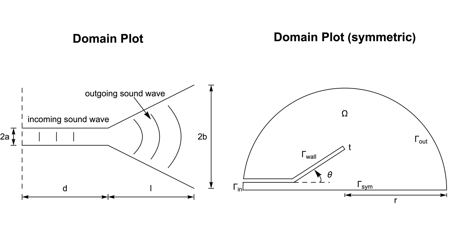
The acoustic horn geometric model consists of two parts: a semi-infinite sound channel with width ![]() and a conical termination with width
and a conical termination with width ![]() at the free end. The geometry is assumed to be infinite in the direction normal to the plane, which reduces the model into a two-dimensional simulation.
at the free end. The geometry is assumed to be infinite in the direction normal to the plane, which reduces the model into a two-dimensional simulation.
Due to the symmetry along the ![]() axis, it is efficient to construct the simulation domain
axis, it is efficient to construct the simulation domain ![]() with only the upper half of the horn, where
with only the upper half of the horn, where ![]() and
and ![]() denote the inlet and outlet boundary. The wall boundary and the symmetric boundary are symbolized as
denote the inlet and outlet boundary. The wall boundary and the symmetric boundary are symbolized as ![]() and
and ![]() , respectively.
, respectively.
t = a / 2;
θ = ArcTan[(b - a) / l];
parametersRules = {r -> 1, a -> 1 / 15, b -> 3 / 10, l -> 1 / 2, d -> 1 / 2};rec1 = Rectangle[{-r, a}, {-r + d, a + t}];
rec2 = Polygon@@(RotationTransform[θ, {-r + d, a}][#]& /@ (List@@RegionBoundary[Rectangle[{-r + d, a}, {-r + d + l / Cos[θ], a + t}]]));
Ω = RegionDifference[Disk[{0, 0}, r, {0, π}], RegionUnion[rec1, rec2]] /. parametersRules;In acoustics simulations, the wavelength ![]() of a sound wave needs to be resolved by a sufficiently fine mesh in order to get an accurate numerical solution. Here the max edge length is set to 12 nodes per
of a sound wave needs to be resolved by a sufficiently fine mesh in order to get an accurate numerical solution. Here the max edge length is set to 12 nodes per ![]() , which means that there will be at least 12 elements per wavelength
, which means that there will be at least 12 elements per wavelength ![]() in each direction of the wave propagation.
in each direction of the wave propagation.
λ = (c / Subscript[f, max]) /. {c -> Subscript[c, air], Subscript[f, max] -> 1000};
h = λ / 12;mesh = ToElementMesh[Ω, MaxCellMeasure -> {"Length" -> h}]Boundary Conditions
There are three types of the boundary conditions involved in this example. At the sound inlet ![]() , a radiation boundary condition is used to model the incoming sound wave.
, a radiation boundary condition is used to model the incoming sound wave.
inlet = Circle[{0, 0}, r, {π - ArcSin[(a/r)], π}] /. parametersRules;
Subscript[Γ, in] = AcousticRadiationValue[{x, y}∈inlet, vars, pars, <|"SoundIncidentPressure" -> 1|>];
On the outer boundary ![]() , an absorbing boundary condition is specified to model the outgoing cylindrical wave.
, an absorbing boundary condition is specified to model the outgoing cylindrical wave.
outlet = Circle[{0, 0}, r, {0, π - ArcSin[(a + t/r)]}] /. parametersRules;Subscript[Γ, out] = AcousticAbsorbingValue[{x, y}∈outlet, vars, pars, <|"AcousticSourceDistance" -> 1 / (2r)|>] /. parametersRules;On the wall boundary ![]() and the symmetric boundary
and the symmetric boundary ![]() , a default sound hard boundary condition is implicitly used.
, a default sound hard boundary condition is implicitly used.
Solve the PDE Model
To analyze the performance of the acoustic horn over the frequency range ![]() , the PDE model is solved repetitively with ParametricNDSolveValue.
, the PDE model is solved repetitively with ParametricNDSolveValue.
pde = FrequencyAcousticsModel == Subscript[Γ, in] + Subscript[Γ, out]fRange = Table[f, {f, 50, 1000, 10}];
pfun = ParametricNDSolveValue[pde, p, {x, y}∈mesh, {ω}];
Monitor[pfunTable = Table[pfun[ω] /. {ω -> 2π f}, {f, fRange}], Row[{"frequency being solved = ", CForm[f], " Hz"}]];Post-processing and Visualization
Sound Pressure Distribution
To visualize the sound propagation within the acoustic horn, the solution is transformed into the time domain with the harmonic wave relation (2):
More information on the relation between the time domain and frequency domain can be found here.
f = 900;
{index} = Flatten[Position[fRange, f]];pMax = Max[Abs[pfunTable[[index]]["ValuesOnGrid"]]];
legendBar = BarLegend[{"TemperatureMap", {-pMax, pMax}}, ...];
options = {PlotRange -> {-pMax, pMax}, ...};boundaryHighlight = Graphics[{...}] /. parametersRules;
nframes = 50;
frames = Table[Show[Legended[ContourPlot[Re[pfunTable[[index]][x, y] * Exp[I ω t] /. {ω -> 2π f}], {x, y}∈Ω, Evaluate[options]], legendBar], boundaryHighlight], {t, 0, 0.002, 0.002 / nframes}];
frames = Rasterize[#1, "Image", ImageResolution -> 80]& /@ frames;
ListAnimate[...]See this note about improving the visual quality of the animation.
As explained in the acoustics tutorial, if the acoustic impedance of two media are inconsistent, then part of the sound wave will be reflected at the interface. The acoustic horn serves as a transformer that matches the impedance between the waveguide ![]() and the surrounding air
and the surrounding air ![]() , so that the reflected sound wave is reduced [3]. The remaining reflected wave results in a flickering sound pressure pattern within the wave channel.
, so that the reflected sound wave is reduced [3]. The remaining reflected wave results in a flickering sound pressure pattern within the wave channel.
Next, a curved acoustic horn is analyzed as a comparison. By smoothing the shape of the horn, the wave reflection can be further minimized.
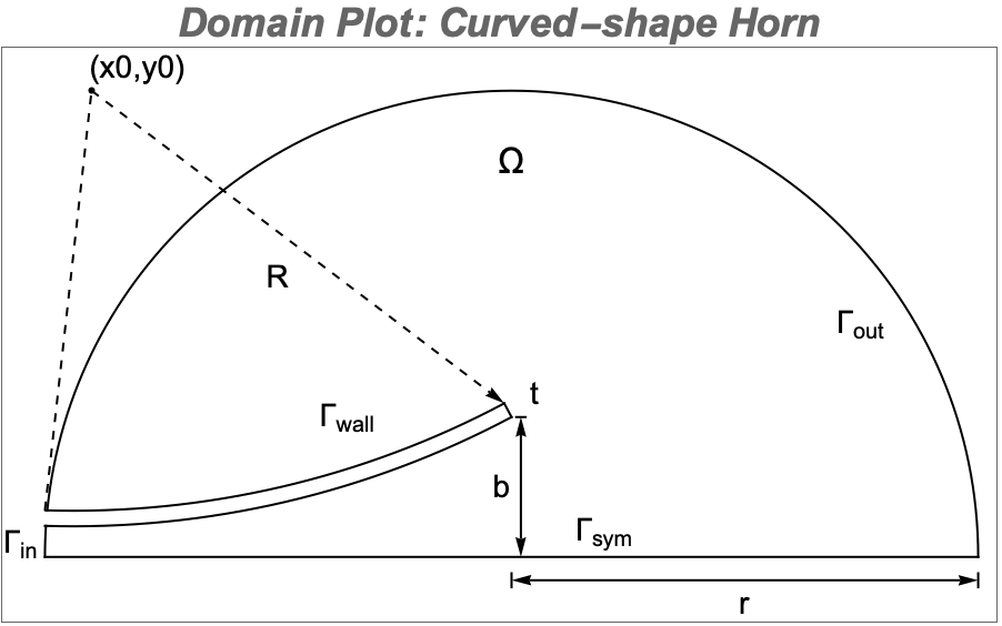
R = 2;
{x0, y0} = {x, y} /. Last[NSolve[{x^2 + (y - b)^2 == R^2, (x + r)^2 + (y - a)^2 == R^2}, {x, y}]];
ϕ = VectorAngle[{-r - x0, a - y0}, {-x0, b - y0}];
γ = (3/2)π - VectorAngle[{0, -1}, {-r - x0, a - y0}];
curve = Annulus[{x0, y0}, {R - t, R}, {γ, γ + ϕ}];
Ωcur = RegionDifference[Disk[{0, 0}, r, {0, π}], curve] /. parametersRules;meshCur = ToElementMesh[Ωcur, MaxCellMeasure -> {"Length" -> h}]pfun2 = ParametricNDSolveValue[pde, p, {x, y}∈meshCur, {ω}];
Monitor[pfunTable2 = Table[pfun2[ω] /. {ω -> 2π f}, {f, fRange}], Row[{"frequency being solved = ", CForm[f], " Hz"}]];boundaryHighlight = Graphics[{...}] /. parametersRules;
nframes = 50;
frames = Table[Show[Legended[ContourPlot[Re[pfunTable2[[index]][x, y] * Exp[I ω t] /. {ω -> 2π f}], {x, y}∈Ωcur, Evaluate[options]], legendBar], boundaryHighlight], {t, 0, 0.002, 0.002 / nframes}];
frames = Rasterize[#1, "Image", ImageResolution -> 80]& /@ frames;
ListAnimate[...]See this note about improving the visual quality of the animation.
In contrast to the rectangular acoustic horn, the curve-shaped boundary has smoothed the gradient of the sound impedance.
The following section demonstrates the procedure to quantify the sound reflection of an acoustic horn.
Index of Reflection Intensity (IRI)
One quantity for measuring the performance of an acoustic horn is the index of reflection intensity (IRI), which is defined as the absolute value of the average reflected wave at the sound inlet ![]() . The formula of the reflection intensity are given by:
. The formula of the reflection intensity are given by:
Subscript[L, in] = N@ArcLength[inlet];Jrec = Table[(Abs[NIntegrate[pfunTable[[i]][x, y], {x, y}∈inlet] / Subscript[L, in] - 1]), {i, fRange//Length}];
Jcur = Table[(Abs[NIntegrate[pfunTable2[[i]][x, y], {x, y}∈inlet] / Subscript[L, in] - 1]), {i, fRange//Length}];ListLogPlot[{Callout[Transpose[{fRange, Jrec}], ...], Callout[Transpose[{fRange, Jcur}], ...]}, ...]As expected, the curved horn has a better performance over most frequencies. Note that the reflection spectrum appears in a decaying pattern with few deep dips, which implies that the acoustic horn is more efficient at higher frequencies. The dips correspond to the resonance frequencies of the acoustic horn, where the sound transmission is further enhanced. The specific frequencies at which the sound resonates are known as the "eigenfrequencies". Advanced designs such as exponential horns and multicell horns [4] can be utilized to improve the horn efficiency at lower frequencies.
Nomenclature
| Symbol | Description | Unit |
| ρ | density of a medium | [kg/m3] |
| c | speed of sound in a medium | [m/s] |
| p | sound pressure | [Pa] |
| ω | sound wave angular frequency | [rad/s] |
| f | sound wave frequency | [Hz] |
| X | position vector | [m] |
| a, b, l, d | geometry parameters | [m] |
| Γin | inlet boundary | N/A |
| Γsym | symmetric boundary | N/A |
| Γwall | wall boundary | N/A |
| Γout | far-field boundary | N/A |
| Ω | computational domain | N/A |
| θ | flare angle of acoustic horn | [rad] |
| J | reflection intensity | [m] |
References
1. E. Bängtsson, D. Noreland and M. Berggren. "Shape Optimization of an Acoustic Horn." Computational Methods in Applied Mechanics and Engineering 192(11–12), 2003 pp. 1533–1571.
2. F. Negri, A. Manzoni and D. Amsallem. "Efficient Model Reduction of Parametrized Systems by Matrix Discrete Empirical Interpolation." Journal of Computational Physics 303, 2015 pp. 431–454.
3. B. Kolbrek. "Horn Theory: An Introduction, Part 1." audioXpress, 2008 pp. 1–8.