Shrink Fitting of Assembly
| Introduction | Solve the PDE Model |
| Domain | Post-processing and Visualization |
| Mesh Generation | Nomenclature |
| Heat Transfer Model | References |
| Initial and Boundary Conditions |
Introduction
Shrink fitting is a manufacturing technique that is used to assemble two metal parts. This is achieved by heating one of the components and cooling the second. Through the induced thermal contraction and expansion, the pieces can be fitted together. After the assembly, the pieces are allowed to return to the ambient temperature, which will in result in the heated piece shrinking while the cooled part expands. If the heated part encloses the cooled part, the assembly will hold together.
In this model, a tungsten rod is to be fitted into a steel frame. The steel frame is slightly widened by preheating it, so that the cooled-down rod can be slipped into the frame. Then the frame gradually contracts and the rod expands as the two parts reach the same ambient temperature, which makes the joint strained and strong.
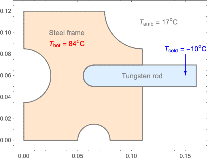
The evolution of the temperature field during the fitting process is simulated with a heat transfer model. The simulation starts with an initial temperature of the steel frame of ![]() and the cooled-down tungsten rod at
and the cooled-down tungsten rod at ![]() . During the shrinking process, both the rod and the steel frame are exposed to the surrounding medium with a temperature
. During the shrinking process, both the rod and the steel frame are exposed to the surrounding medium with a temperature ![]() and respectively gain and lose heat through thermal convection during the time of the assembly process. This process will be modeled. From the simulation, the time
and respectively gain and lose heat through thermal convection during the time of the assembly process. This process will be modeled. From the simulation, the time ![]() required to fit the rod and the frame can be estimated.
required to fit the rod and the frame can be estimated.
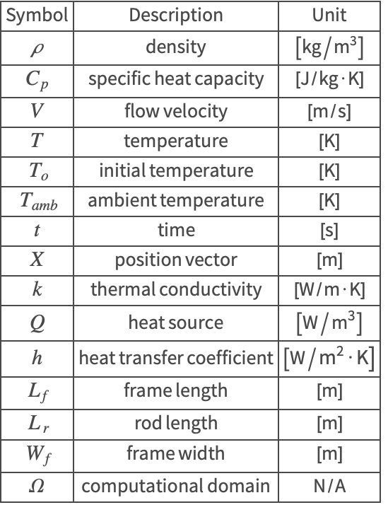
The symbols and corresponding units used here are summarized in the Nomenclature section.
Please refer to the information provided in"Heat Transfer" for a more general theoretical background for heat transfer analysis.
Needs["NDSolve`FEM`"]Domain
The dimensions of the simulation domain ![]() are illustrated in the following plots:
are illustrated in the following plots:
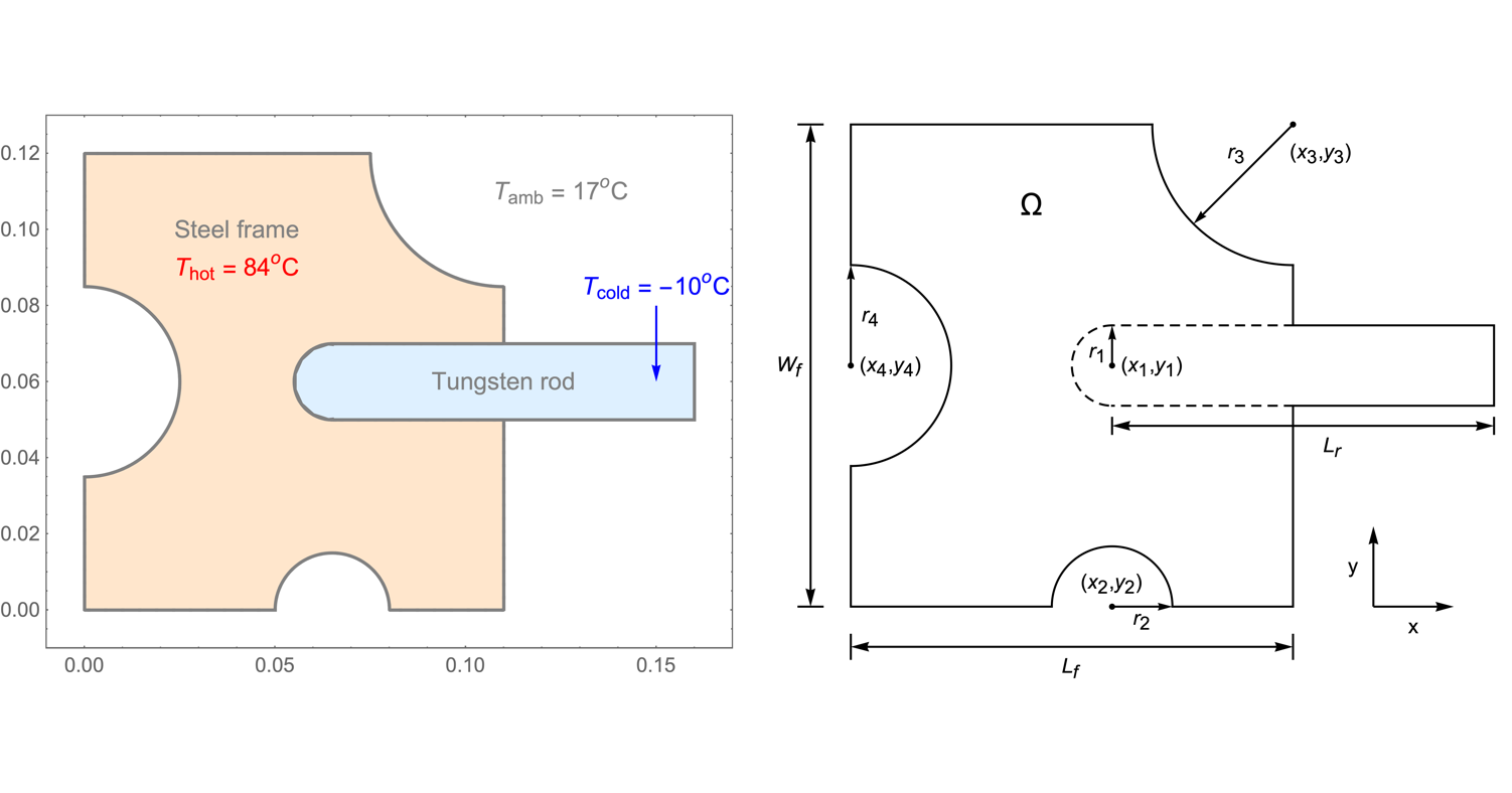
Subscript[L, f] = 0.11;Subscript[W, f] = 0.12;Subscript[L, r] = 0.095;
r1 = 0.01;x1 = 0.065;y1 = 0.06;
r2 = 0.015;x2 = 0.065;y2 = 0;
r3 = 0.035;x3 = 0.11;y3 = 0.12;
r4 = 0.025;x4 = 0;y4 = 0.06;rod = RegionUnion[Rectangle[{x1, y1 - r1}, {x1 + Subscript[L, r], y1 + r1}], Disk[{x1, y1}, r1]];
frame = RegionDifference[RegionDifference[Rectangle[{0, 0}, {Subscript[L, f], Subscript[W, f]}], RegionUnion[Disk[{x2, y2}, r2], Disk[{x3, y3}, r3], Disk[{x4, y4}, r4]]], rod];Ω = RegionUnion[rod, frame];Mesh Generation
A simple way to generate the mesh is by discretizing the whole domain directly. However, in that case, the interface between the rod and frame (marked in red) is not preserved, which may reduce the accuracy of the simulation.
bounds = 1.1 * {{0, x1 + Subscript[L, r]}, {0, Subscript[W, f]}};
mesh = ToElementMesh[Ω, bounds];Show[mesh["Wireframe"], Graphics[{...}]]An easy way to preserve the internal boundary between the rod and frame when creating the mesh is to make use of the function BoundaryElementMeshJoin. This function is provided by the FEMAddOns paclet, which can conveniently be installed with the resource function FEMAddOnsInstall.
The first step is to create the boundary element mesh for the rod and steel frame separately.
Subscript[bm, f] = ToBoundaryMesh[frame, bounds];
Subscript[bm, r] = ToBoundaryMesh[Line[{{Subscript[L, f], y1 - r1}, {x1 + Subscript[L, r], y1 - r1}, {x1 + Subscript[L, r], y1 + r1}, {Subscript[L, f], y1 + r1}}]];ResourceFunction["FEMAddOnsInstall"][]Needs["FEMAddOns`"]bmesh = FEMUtils`BoundaryElementMeshJoin[Subscript[bm, f], Subscript[bm, r]]Next, different markers are assigned to the rod and frame. These markers can then be used to set up the material parameters (![]() ,
, ![]() and
and ![]() ). Using markers for this is much simpler than specifying the formula for each subregion. More information on markers and their generation in meshes can be found in the "Element Mesh Generation" tutorial.
). Using markers for this is much simpler than specifying the formula for each subregion. More information on markers and their generation in meshes can be found in the "Element Mesh Generation" tutorial.
For markers to be attributed to different subregions, coordinates that lie in those subregions need to be specified.
rodCoordinate = {0.11, 0.06};
frameCoordinate = {0.05, 0.1};
Visualizing the boundary mesh and the marker coordinates helps one understand the process of specifying marker coordinates. For the visualization, it is necessary to group the marker coordinates and set up colors that will go with the markers.
markerColors = {Blue, Orange};
markerCoordinates = {{rodCoordinate}, {frameCoordinate}};Show[{bmesh["Wireframe"], Graphics[MapThread[{PointSize[0.02], #1, Point /@ #2}&, {markerColors, markerCoordinates}]]}]region = <|"rod" -> 1, "frame" -> 2|>;Now the full element mesh can be generated. In order to get a good result, a grid finer than the default is used for the mesh generation.
markerSpecification = {{rodCoordinate, region["rod"]}, {frameCoordinate, region["frame"]}};mesh = ToElementMesh[bmesh, "RegionMarker" -> markerSpecification, "MaxCellMeasure" -> 5 * 10^-6];
GraphicsRow[{mesh["Wireframe"[Rule[...]]], mesh["Wireframe"[...]]}]Note that the internal boundary between the rod and frame is preserved.
Now the material parameters can be set up using ElementMarker.
Heat Transfer Model
The heat equation (1) is used to solve for the temperature field in a heat transfer model:
For a transient heat transfer model without sources, the source term ![]() in (2) is set to zero. Since a solid is modeled, any internal velocity
in (2) is set to zero. Since a solid is modeled, any internal velocity ![]() also vanishes, and the heat equation simplifies to:
also vanishes, and the heat equation simplifies to:
vars = {T[t, x, y], t, {x, y}};
HeatTransferPDEComponent[vars, <|"MassDensity" -> ρ, "SpecificHeatCapacity" -> Subscript[C, p], "ThermalConductivity" -> k|>]pars = <||>;
pars["MassDensity"] = If[ElementMarker == region["rod"], Subscript[ρ, tungsten], Subscript[ρ, steel]];
pars["SpecificHeatCapacity"] = If[ElementMarker == region["rod"], Subscript[Cp, tungsten], Subscript[Cp, steel]];
pars["ThermalConductivity"] = If[ElementMarker == region["rod"], Subscript[k, tungsten], Subscript[k, steel]] * IdentityMatrix[2];pars[Subscript[ρ, tungsten]] = 19000;
pars[Subscript[Cp, tungsten]] = 134;
pars[Subscript[k, tungsten]] = 163;
pars[Subscript[ρ, steel]] = 7500;
pars[Subscript[Cp, steel]] = 470;
pars[Subscript[k, steel]] = 44;op = HeatTransferPDEComponent[vars, pars]Also, see this note about how to set up computationally efficient PDE coefficients. Note that in this case, the symbolic names of the material properties have been replaced by the actual values given. This is because the PDEComponents function replaces these parameters.
Initial and Boundary Conditions
Prior to the assembly, the rod and the frame are maintained at ![]() and
and ![]() .
.
Subscript[T, cold] = -10;
Subscript[T, hot] = 84;
Subscript[T, amb] = 17;
ic = {T[0, x, y] == Piecewise[{
	{Subscript[T, cold], ElementMarker == region["rod"]}, {Subscript[T, hot], ElementMarker == region["frame"]}}]};
All the external boundaries are exposed to thermal convection with the surrounding medium. The heat transfer coefficient and the ambient temperature are given by ![]() and
and ![]() , respectively.
, respectively.
Subscript[Γ, convective] = HeatTransferValue[Not[(x1 - r1 ≤ x < Subscript[L, f]) && (y1 - r1 ≤ y ≤ y1 + r1)], vars, pars, <|"AmbientTemperature" -> Subscript[T, amb], "HeatTransferCoefficient" -> 500|>]Here, the external boundary is specified by excluding the region that involves the internal boundary.
Solve the PDE Model
To analyze the heat flow between the assembled rod and frame, the PDE model is solved from ![]() to
to ![]() .
.
tend = 200;pde = {op == Subscript[Γ, convective], ic};measure = AbsoluteTiming[MaxMemoryUsed[Monitor[Tfun = NDSolveValue[pde, T, {t, 0, tend}, {x, y}∈mesh, EvaluationMonitor :> (monitor = Row[{"t = ", CForm[t]}])], monitor]] / (1024. ^ 2)];
Print["Time -> ", measure[[1]], "
Memory -> ", measure[[2]]]Post-processing and Visualization
To inspect the effect of the shrink fitting, the temperature distribution ![]() is visualized evolving in time.
is visualized evolving in time.
TRange = 1.1 * {Subscript[T, cold], Subscript[T, hot]};
legendBar = BarLegend[{"TemperatureMap", TRange}, ...];
options = {PlotRange -> TRange, ...};boundaryHighlight = Graphics[{...}];
frames = Table[Labeled[Show[Legended[
ContourPlot[Tfun[t, x, y], {x, y}∈mesh, Evaluate[options]], legendBar], boundaryHighlight], Text[...]], {t, PowerRange[0.1, tend, 1.25]}];
frames = Rasterize[#1, "Image", ImageResolution -> 80]& /@ frames;
ListAnimate[...]See this note about improving the visual quality of the animation.
Now a rough estimate is made ![]() on how long the fitting process takes. The estimate is rough because a full structural mechanics thermal expansion model has not been made use of. Instead, a simple assumption is made. An initial gap of
on how long the fitting process takes. The estimate is rough because a full structural mechanics thermal expansion model has not been made use of. Instead, a simple assumption is made. An initial gap of ![]() between the steel frame and the tungsten rod is assumed and the material's thermal expansion coefficients is used to determine the time
between the steel frame and the tungsten rod is assumed and the material's thermal expansion coefficients is used to determine the time ![]() it takes to fit the rod and the frame.
it takes to fit the rod and the frame.
First, at each time step, the maximum temperature ![]() (of the steel frame) and the minimum temperature
(of the steel frame) and the minimum temperature ![]() (of the rod) are retrieved.
(of the rod) are retrieved.
timeStep = Tfun["Coordinates"][[1]];
steps = timeStep//Length;
MaxPts = Table[{timeStep[[i]], Max[Tfun["ValuesOnGrid"][[i]]]}, {i, 1, steps}];
MinPts = Table[{timeStep[[i]], Min[Tfun["ValuesOnGrid"][[i]]]}, {i, 1, steps}];
Tmax = Interpolation[MaxPts];
Tmin = Interpolation[MinPts];
Plot[{Tmax[t], Tmin[t]}, {t, 0, tend}, ...]
The thermal expansion/contraction effect is described by equation (3). Here ![]() and
and ![]() are the thermal expansion coefficients for the steel frame and the tungsten rod:
are the thermal expansion coefficients for the steel frame and the tungsten rod:
Based on the gap ![]() between the frame and the rod, it is then possible to solve for the time
between the frame and the rod, it is then possible to solve for the time ![]() in which the gap will be filled (i.e.
in which the gap will be filled (i.e. ![]() ).
).
FindRoot[δ == L * (Subscript[α, steel](Subscript[T, hot] - Tmax[t]) + Subscript[α, tungsten](Tmin[t] - Subscript[T, cold]))
	 /. {δ -> 1.2 * 10^-5, L -> 2 * r1, Subscript[α, steel] -> 1.2 * 10^-5, Subscript[α, tungsten] -> 4.5 * 10^-6}, {t, 1}]
During the assembly, the heat flow between the hot frame and the cold rod slowly converges the temperatures ![]() and
and ![]() . The change in temperature makes the frame contract and the rod expand, which eventually binds the two components in place. It is estimated that the frame and the rod will be fitted together roughly at
. The change in temperature makes the frame contract and the rod expand, which eventually binds the two components in place. It is estimated that the frame and the rod will be fitted together roughly at ![]() .
.
Nomenclature
References
1. Krysl, P. A Pragmatic Introduction to the Finite Element Method for Thermal and Stress Analysis. Pressure Cooker Press. (2005).