Wolfram Language & System Documentation Center

AsymptoticEqual

AsymptoticEqual[f,g,xx^*]

gives conditions for or as xx^*.

AsymptoticEqual[f,g,{x₁,…,x_n}{,…,}]

gives conditions for or as {x₁,…,x_n}{,…,}.

Details and Options

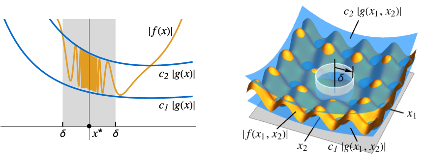
Asymptotic equal is also expressed as f is big-theta of g, f is bounded by g, f is of order g, and f grows as g. The point x^* is often assumed from context.
Asymptotic equal is an equivalence relation and means $c_1 TemplateBox[{{g, (, x, )}}, Abs]<=TemplateBox[{{f, (, x, )}}, Abs]<=c_2 TemplateBox[{{g, (, x, )}}, Abs]$ when x is near x^* for some constants and . It is a coarser asymptotic equivalence relation than AsymptoticEquivalent.
Typical uses include expressing simple bounds for functions and sequences near some point. It is frequently used for asymptotic solutions to equations and to give simple lower bounds for computational complexity.
For a finite limit point x^* and {,…,}, the result is:

	AsymptoticEqual[f[x],g[x],xx^*]	there exist , and such that $0<TemplateBox[{{x, -, {x, ^, }}}, Abs]<delta(c_1,c_2,x^)$ implies $c_1 TemplateBox[{{g, (, x, )}}, Abs]<=TemplateBox[{{f, (, x, )}}, Abs]<=c_2 TemplateBox[{{g, (, x, )}}, Abs]$
	AsymptoticEqual[f[x₁,…,x_n],g[x₁,…,x_n],{x₁,…,x_n}{,…,}]	there exist , and such that $0<TemplateBox[{{{, {{{x, _, 1}, -, {x, _, {(, 1, )}, ^, }}, ,, ..., ,, {{x, _, n}, -, {x, _, {(, n, )}, ^, }}}, }}}, Norm]<delta(epsilon,x^*)$ implies $c_1 TemplateBox[{{g, (, {{x, _, 1}, ,, ..., ,, {x, _, n}}, )}}, Abs]<=TemplateBox[{{f, (, {{x, _, 1}, ,, ..., ,, {x, _, n}}, )}}, Abs]<=c_2 TemplateBox[{{g, (, {{x, _, 1}, ,, ..., ,, {x, _, n}}, )}}, Abs]$

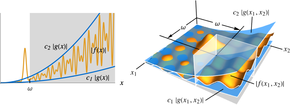
For an infinite limit point, the result is:

	AsymptoticEqual[f[x],g[x],x∞]	there exist , and such that implies $c_1 TemplateBox[{{g, (, x, )}}, Abs]<=TemplateBox[{{f, (, x, )}}, Abs]<=c_2 TemplateBox[{{g, (, x, )}}, Abs]$
	AsymptoticEqual[f[x₁,…,x_n],g[x₁,…,x_n],{x₁,…,x_n}{∞,…,∞}]	there exist , and such that implies $c_1 TemplateBox[{{g, (, {{x, _, 1}, ,, ..., ,, {x, _, n}}, )}}, Abs]<=TemplateBox[{{f, (, {{x, _, 1}, ,, ..., ,, {x, _, n}}, )}}, Abs]<=c_2 TemplateBox[{{g, (, {{x, _, 1}, ,, ..., ,, {x, _, n}}, )}}, Abs]$

AsymptoticEqual[f[x],g[x],xx^*] exists if and only if MinLimit[Abs[f[x]/g[x]],xx^*]>0 and MaxLimit[Abs[f[x]/g[x]],xx^*]<∞ when g[x] does not have an infinite set of zeros near x^*.
The following options can be given:

Assumptions	$Assumptions	assumptions on parameters
Direction	Reals	direction to approach the limit point
GenerateConditions	Automatic	generate conditions for parameters
Method	Automatic	method to use
PerformanceGoal	"Quality"	what to optimize

Possible settings for Direction include:

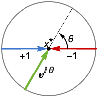
	Reals or "TwoSided"	from both real directions
	"FromAbove" or -1	from above or larger values
	"FromBelow" or +1	from below or smaller values
	Complexes	from all complex directions
	Exp[ θ]	in the direction
	{dir₁,…,dir_n}	use direction dir_i for variable x_i independently

DirectionExp[ θ] at x^* indicates the direction tangent of a curve approaching the limit point x^*.

Possible settings for GenerateConditions include:
Automatic non-generic conditions only

True all conditions

False no conditions

None return unevaluated if conditions are needed
Possible settings for PerformanceGoal include $PerformanceGoal, "Quality" and "Speed". With the "Quality" setting, Limit typically solves more problems or produces simpler results, but it potentially uses more time and memory.

Examples

open all close all

Basic Examples (2)

Verify that as :

The former can be "sandwiched" between two constant multiples of the latter:

Verify that as :

The former can be "sandwiched" between two constant multiples of the latter:

Scope (9)

Compare functions that are not strictly positive:

Show that diverges at the same rate as at the origin:

Answers may be Boolean expressions rather than explicit True or False:

When comparing functions with parameters, conditions for the result may be generated:

By default, a two-sided comparison of the functions is made:

When comparing larger values of , vanishes at the same rate as $x^2(1-cos(x)) TemplateBox[{{x}}, UnitStepSeq]$ :

The relationship fails for smaller values of :

Visualize the ratio of the two functions, showing it approaches a nonzero limit from above:

Functions like Sqrt may have the same relationship in both real directions along the negative reals:

If approached from above in the complex plane, the same relationship is observed:

However, approaching from below in the complex plane produces a different result:

This is due to a branch cut where the imaginary part of Sqrt reverses sign as the axis is crossed:

Hence, the relationship does not hold in the complex plane in general:

Visualize the relative sizes of the functions when approached from the four real and imaginary directions:

Compare multivariate functions:

Visualize the norms of the two functions:

Compare multivariate functions at infinity:

Use parameters when comparing multivariate functions:

Options (9)

Assumptions (1)

Specify conditions on parameters using Assumptions:

Different assumptions can produce different results:

Direction (5)

Equality from below:

Equivalently:

Equality from above:

Equivalently:

Equality at piecewise discontinuities:

Since it fails in one direction, the two-sided result is false as well:

Visualize the two functions and their ratio:

Equality at a pole is independent of the direction of approach:

Equality at a branch cut:

Compute equality, approaching from different quadrants:

Approaching the origin from the third quadrant:

Equivalently:

Approaching the origin from the second quadrant:

Approaching the origin from the right half-plane:

Approaching the origin from the bottom half-plane:

Visualize the ratio of the functions:

GenerateConditions (3)

Return a result without stating conditions:

This result is only valid if n>0:

Return unevaluated if the results depend on the value of parameters:

By default, conditions are not generated if only special values invalidate the result:

With GenerateConditions->True, even these non-generic conditions are reported:

Applications (10)

Basic Applications (5)

Show that two monomials equivalent at infinity have the same power:

Use this to show that two polynomials that are equivalent are of the same order:

Visualize the ratios of three pairs of asymptotically equivalent polynomials:

Show that two monomials in equivalent at have the same power:

Use this to show that two polynomials in that are equivalent have the same leading monomial:

Visualize the ratios of three pairs of asymptotically equivalent polynomials in :

Show that at :

Visualize the functions:

Even though the absolute value of their ratio wiggles incessantly as , it is bounded away from :

Show that :

Even though the absolute value of their ratio wiggles incessantly as , it is bounded away from :

Show that at :

Computational Complexity (3)

In a bubble sort, adjoining neighbors are compared and swapped if they are out of order. After one pass of n-1 comparisons, the largest element is at the end. The process is then repeated on remaining n-1 elements, and so forth, until only two elements at the very beginning remain. If comparison and swap takes c steps, the total number of steps for the sort is as follows:

Show that , and thus the algorithm has quadratic run time:

Visualize the ratios for the two functions for different values of c:

In a merge sort, the list of elements is split in two, each half is sorted, and then the two halves are combined. Thus, the time T[n] to do the sort will be the sum of some constant time b to compute the middle, 2T[n/2] to sort each half, and some multiple a n of the number of elements to combine the two halves:

Solve the recurrence equation to find the time t to sort n elements:

Show that , and thus the algorithm has run time:

Strassen's algorithm was the first subcubic matrix multiplication algorithm found. It consists of four steps: splitting each of the two matrices into 4 equal-sized submatrices, forming 14 particular linear combinations out of the 8 submatrices, multiplying 7 pairs of these and forming linear combinations of the 7 results. The time to do the multiplication will therefore be a constant time to split the matrix, for forming linear combinations in the second and fourth steps and for the third step:

Solve the recurrence relation:

Though the result is complicated, it is asymptotically equal to :

Compare the rate of growth of the naive cubic algorithm and Strassen's algorithm:

Convergence Testing (2)

A sequence is said to be absolutely summable if $sum_(n=1)^inftyTemplateBox[{{a, _, n}}, Abs]<infty$ . If a second sequence , the comparison test states that is absolutely summable if and only if is. Use the test to show that converges by comparing with the sum of :

Compare with the answer given by SumConvergence:

Show that convergence by comparing with the sum of :

Show that divergence by comparing with the sum of :

Compare with the answer given by SumConvergence:

The sequence , and thus is not absolutely summable:

A function is said to be absolutely integrable on if $int_a^bTemplateBox[{{f, , {(, x, )}}}, Abs]dx<infty$ . If and are continuous on the open interval and at both and , the comparison test states that is absolutely integrable if and only if is. Use the test to show that is absolutely integrable on :