ElectricCurrentDensityValue[pred,vars,pars]
represents a current density boundary condition for PDEs with predicate pred indicating where it applies, with model variables vars and global parameters pars.
ElectricCurrentDensityValue[pred,vars,pars,lkey]
represents a current density boundary condition with local parameters specified in pars[lkey].


ElectricCurrentDensityValue
ElectricCurrentDensityValue[pred,vars,pars]
represents a current density boundary condition for PDEs with predicate pred indicating where it applies, with model variables vars and global parameters pars.
ElectricCurrentDensityValue[pred,vars,pars,lkey]
represents a current density boundary condition with local parameters specified in pars[lkey].
Details


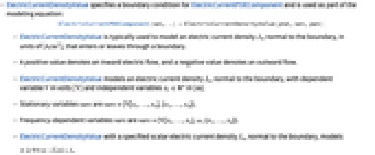
- ElectricCurrentDensityValue specifies a boundary condition for ElectricCurrentPDEComponent and is used as part of the modeling equation:
- ElectricCurrentDensityValue is used to model an electric current density
 in [
in [![TemplateBox[{InterpretationBox[, 1], {"A", , "/", , {"m", ^, 2}}, amperes per meter squared, {{(, "Amperes", )}, /, {(, {"Meters", ^, 2}, )}}}, QuantityTF] TemplateBox[{InterpretationBox[, 1], {"A", , "/", , {"m", ^, 2}}, amperes per meter squared, {{(, "Amperes", )}, /, {(, {"Meters", ^, 2}, )}}}, QuantityTF]](Files/ElectricCurrentDensityValue.en/3.png) ], normal to the boundary, that enters or leaves through a boundary.
], normal to the boundary, that enters or leaves through a boundary. - A positive value denotes an inward electric flow, and a negative value denotes an outward flow.
- ElectricCurrentDensityValue models an electric current density
 , normal to the boundary, with dependent variable
  in volts [
![TemplateBox[{InterpretationBox[, 1], "V", volts, "Volts"}, QuantityTF] TemplateBox[{InterpretationBox[, 1], "V", volts, "Volts"}, QuantityTF]](Files/ElectricCurrentDensityValue.en/6.png) ] and independent variables
] and independent variables  in [
in [![TemplateBox[{InterpretationBox[, 1], "m", meters, "Meters"}, QuantityTF] TemplateBox[{InterpretationBox[, 1], "m", meters, "Meters"}, QuantityTF]](Files/ElectricCurrentDensityValue.en/8.png) ].
]. - Stationary variables vars are vars={V[x1,…,xn],{x1,…,xn}}.
- Frequency-dependent variables vars are vars={V[x1,…,xn],ω,{x1,…,xn}}.
- ElectricCurrentDensityValue with a specified scalar electric current density
 , normal to the boundary, models:
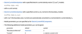
 - ElectricCurrentDensityValue with a specified electric current density vector
 [
[![TemplateBox[{InterpretationBox[, 1], {"A", , "/", , {"m", ^, 2}}, amperes per meter squared, {{(, "Amperes", )}, /, {(, {"Meters", ^, 2}, )}}}, QuantityTF] TemplateBox[{InterpretationBox[, 1], {"A", , "/", , {"m", ^, 2}}, amperes per meter squared, {{(, "Amperes", )}, /, {(, {"Meters", ^, 2}, )}}}, QuantityTF]](Files/ElectricCurrentDensityValue.en/12.png) ], models:
], models: - with
 a unit normal.
 - ElectricCurrentDensityValue with a specified current
 [
[![TemplateBox[{InterpretationBox[, 1], "A", amperes, "Amperes"}, QuantityTF] TemplateBox[{InterpretationBox[, 1], "A", amperes, "Amperes"}, QuantityTF]](Files/ElectricCurrentDensityValue.en/16.png) ], normal to the boundary, models:
], normal to the boundary, models: - with
 [
[![TemplateBox[{InterpretationBox[, 1], {{"m", ^, 2}}, meters squared, {"Meters", ^, 2}}, QuantityTF] TemplateBox[{InterpretationBox[, 1], {{"m", ^, 2}}, meters squared, {"Meters", ^, 2}}, QuantityTF]](Files/ElectricCurrentDensityValue.en/19.png) ] the boundary area. Currents are automatically converted to a normal electric current density
] the boundary area. Currents are automatically converted to a normal electric current density  .
. - Model parameters pars are specified as for ElectricCurrentPDEComponent.
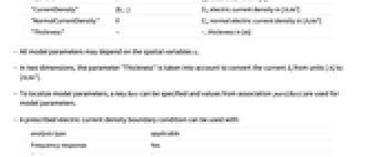
- The following additional model parameters pars can be given:
-
parameter default symbol "BoundaryUnitNormal" Automatic 
"Current" 
 , electric current in [
![TemplateBox[{InterpretationBox[, 1], "A", amperes, "Amperes"}, QuantityTF] TemplateBox[{InterpretationBox[, 1], "A", amperes, "Amperes"}, QuantityTF]](Files/ElectricCurrentDensityValue.en/24.png) ]
]"CurrentDensity" - {0,...}
 , electric current density in [
![TemplateBox[{InterpretationBox[, 1], {"A", , "/", , {"m", ^, 2}}, amperes per meter squared, {{(, "Amperes", )}, /, {(, {"Meters", ^, 2}, )}}}, QuantityTF] TemplateBox[{InterpretationBox[, 1], {"A", , "/", , {"m", ^, 2}}, amperes per meter squared, {{(, "Amperes", )}, /, {(, {"Meters", ^, 2}, )}}}, QuantityTF]](Files/ElectricCurrentDensityValue.en/26.png) ]
]"NormalCurrentDensity" 
 , normal electric current density in [
![TemplateBox[{InterpretationBox[, 1], {"A", , "/", , {"m", ^, 2}}, amperes per meter squared, {{(, "Amperes", )}, /, {(, {"Meters", ^, 2}, )}}}, QuantityTF] TemplateBox[{InterpretationBox[, 1], {"A", , "/", , {"m", ^, 2}}, amperes per meter squared, {{(, "Amperes", )}, /, {(, {"Meters", ^, 2}, )}}}, QuantityTF]](Files/ElectricCurrentDensityValue.en/29.png) ]
]"Thickness" -  , thickness in [
![TemplateBox[{InterpretationBox[, 1], "m", meters, "Meters"}, QuantityTF] TemplateBox[{InterpretationBox[, 1], "m", meters, "Meters"}, QuantityTF]](Files/ElectricCurrentDensityValue.en/31.png) ]
] - All model parameters may depend on the spatial variables
 .
. - In two dimensions, the parameter "Thickness" is taken into account to convert the current
 from units [
![TemplateBox[{InterpretationBox[, 1], "A", amperes, "Amperes"}, QuantityTF] TemplateBox[{InterpretationBox[, 1], "A", amperes, "Amperes"}, QuantityTF]](Files/ElectricCurrentDensityValue.en/34.png) ] to [
] to [![TemplateBox[{InterpretationBox[, 1], {"A", , "/", , {"m", ^, 2}}, amperes per meter squared, {{(, "Amperes", )}, /, {(, {"Meters", ^, 2}, )}}}, QuantityTF] TemplateBox[{InterpretationBox[, 1], {"A", , "/", , {"m", ^, 2}}, amperes per meter squared, {{(, "Amperes", )}, /, {(, {"Meters", ^, 2}, )}}}, QuantityTF]](Files/ElectricCurrentDensityValue.en/35.png) ].
]. - To localize model parameters, a key lkey can be specified and values from association pars[lkey] are used for model parameters.
- A prescribed electric current density boundary condition can be used with:
-
analysis type applicable Frequency response Yes Stationary Yes - ElectricCurrentDensityValue evaluates to a NeumannValue.
- The boundary predicate pred can be specified as in NeumannValue.
- If the ElectricCurrentDensityValue depends on parameters
 that are specified in the association pars as …,keypi…,pivi,…, the parameters
  are replaced with
  .
.
Examples
open all close allBasic Examples (3)
Set up a symbolic electric current density boundary condition:
Set up a symbolic electric current density boundary condition with a current density:
Model a copper wire that is excited with a direct current (DC) of ![]() [
[![]() ] with a current density boundary condition at the lower-left boundary and with a zero electric potential condition at the lower-right boundary.
] with a current density boundary condition at the lower-left boundary and with a zero electric potential condition at the lower-right boundary.
Set up the stationary current PDE model variables ![]() and
and ![]() :
:
Define the geometry of the wire:
Specify ground potential at the lower-right boundary:
Scope (6)
Create an electric current density boundary condition:
Create an electric current density boundary condition with a boundary unit normal ![]() :
:
Create an electric current density boundary condition with ![]() :
:
Create an electric current density boundary condition with a current ![]() :
:
Create an electric current density boundary condition in 2D with a current ![]() and a thickness
and a thickness ![]() :
:
Create a parametric-frequency electric current density boundary condition:
Applications (2)
3D Stationary Analysis (1)
Model a copper spiral inductor that is excited with a current density normal to the left boundary and has a zero electric potential boundary condition at the right boundary.
Define the spiral inductor geometry:
Set up the stationary current PDE model variables ![]() and
and ![]() :
:
Specify an inward current flow on the left boundary:
Frequency Analysis (1)
Model a dielectric material of a cylindrical capacitor that is excited with an alternating current (AC ) of ![]() [
[![]() ], with a current density boundary condition at the upper boundary, which represents one of the capacitor electrodes, and with a zero electric potential boundary condition at the lower boundary.
], with a current density boundary condition at the upper boundary, which represents one of the capacitor electrodes, and with a zero electric potential boundary condition at the lower boundary.
Set up the frequency current PDE model variables ![]() :
:
Define the frequency and the period:
Specify an electrical conductivity ![]() and a relative permittivity
and a relative permittivity ![]() :
:
Specify the ground potential at the lower boundary:
Specify an inward current flow at the upper boundary:
Solve the harmonic PDE for ![]() [
[![]() ]:
]:
Transform the voltage at the upper boundary to the time domain:
Tech Notes
Related Guides
History
Text
Wolfram Research (2024), ElectricCurrentDensityValue, Wolfram Language function, https://reference.wolfram.com/language/ref/ElectricCurrentDensityValue.html.
CMS
Wolfram Language. 2024. "ElectricCurrentDensityValue." Wolfram Language & System Documentation Center. Wolfram Research. https://reference.wolfram.com/language/ref/ElectricCurrentDensityValue.html.
APA
Wolfram Language. (2024). ElectricCurrentDensityValue. Wolfram Language & System Documentation Center. Retrieved from https://reference.wolfram.com/language/ref/ElectricCurrentDensityValue.html
BibTeX
@misc{reference.wolfram_2025_electriccurrentdensityvalue, author="Wolfram Research", title="{ElectricCurrentDensityValue}", year="2024", howpublished="\url{https://reference.wolfram.com/language/ref/ElectricCurrentDensityValue.html}", note=[Accessed: 08-May-2026]}
BibLaTeX
@online{reference.wolfram_2025_electriccurrentdensityvalue, organization={Wolfram Research}, title={ElectricCurrentDensityValue}, year={2024}, url={https://reference.wolfram.com/language/ref/ElectricCurrentDensityValue.html}, note=[Accessed: 08-May-2026]}