HeatTransferPDEComponent

HeatTransferPDEComponent[vars,pars]

yields a heat transfer PDE term with variables vars and parameters pars.

Details

HeatTransferPDEComponent returns a sum of differential operators to be used as a part of partial differential equations:

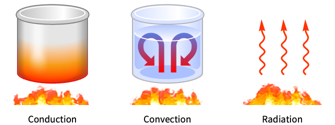
HeatTransferPDEComponent models the generation and propagation of thermal energy in physical systems by mechanisms such as convection, conduction and radiation.

HeatTransferPDEComponent models heat transfer phenomena with dependent variable temperature in [], independent variables in [] and time variable in [].
Stationary variables vars are vars={Θ[x₁,…,x_n],{x₁,…,x_n}}.
Time-dependent variables vars are vars={Θ[t,x₁,…,x_n],t,{x₁,…,x_n}}.
The non-conservative time-dependent heat transfer model HeatTransferPDEComponent is based on a convection-diffusion model with mass density , specific heat capacity , thermal conductivity , convection velocity vector and heat source :

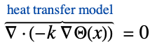
The non-conservative stationary heat transfer PDE term is given by:

The implicit default boundary condition for the non-conservative model is a HeatOutflowValue.
The difference between the non-conservative model and the conservative model is the treatment of a convection velocity .
The units of the heat transfer model terms are in [ $TemplateBox[{InterpretationBox[, 1], {"W", , "/", , {"m", ^, 3}}, watts per meter cubed, {{(, "Watts", )}, /, {(, {"Meters", ^, 3}, )}}}, QuantityTF]$ ], or equivalently in [ $TemplateBox[{InterpretationBox[, 1], {"J", , "/(", , {"m", ^, 3}, , "s", , ")"}, joules per meter cubed second, {{(, "Joules", )}, /, {(, {{"Meters", ^, 3}, , "Seconds"}, )}}}, QuantityTF]$ ].
The following parameters pars can be given:

parameter	default	symbol
"HeatConvectionVelocity"	{0,…}	, flow velocity []
"HeatSource"	0	, heat source [ $TemplateBox[{InterpretationBox[, 1], {"W", , "/", , {"m", ^, 3}}, watts per meter cubed, {{(, "Watts", )}, /, {(, {"Meters", ^, 3}, )}}}, QuantityTF]$ ]
"MassDensity"	1	, density [ $TemplateBox[{InterpretationBox[, 1], {"kg", , "/", , {"m", ^, 3}}, kilograms per meter cubed, {{(, "Kilograms", )}, /, {(, {"Meters", ^, 3}, )}}}, QuantityTF]$ ]
"Material"	Automatic
"ModelForm"	"NonConservative"	none
"RegionSymmetry"	None
"SpecificHeatCapacity"	1	, specific heat capacity []
"ThermalConductivity"	IdentityMatrix	, thermal conductivity [

All parameters may depend on any of , and , as well as other dependent variables.
The number of independent variables determines the dimensions of and the length of .
Sometimes the heat equation is specified with a thermal diffusivity. The thermal diffusivity is the thermal conductivity divided by the density and the specific heat capacity at constant pressure.
The thermal convection velocity specifies the velocity with which a fluid transports heat. If no fluid is present, the thermal convection velocity is 0.
A heat source models thermal energy that is introduced (positive) or removed (negative) from the system.
A possible choice for the parameter "RegionSymmetry" is "Axisymmetric".
"Axisymmetric" region symmetry represents a truncated cylindrical coordinate system where the cylindrical coordinates are reduced by removing the angle variable as follows:
dimension reduction equation

1D

2D
The input specification for the parameters is exactly the same as for their corresponding operator terms.
Coupled equations can be generated with the same input specification as with the corresponding operator terms.
If no parameters are specified, the default heat transfer PDE is:

If the HeatTransferPDEComponent depends on parameters that are specified in the association pars as …,keyp_i…,p_iv_i,…], the parameters are replaced with .

Examples

open allclose all

Basic Examples (4)

Define a time-independent heat transfer model:

Define a time-dependent heat transfer model:

Set up a time-dependent heat transfer model with particular material parameters:

Model a temperature field with a heat source in a rod:

Solve the PDE:

Visualize the solution:

Scope (7)

Set up a time-dependent heat transfer model for a particular material:

Set up a time-dependent heat transfer model for several material regions:

1D (1)

Model a temperature field with two heat conditions at the sides:

Set up the heat transfer model variables :

Set up a region :

Specify heat transfer model parameter thermal conductivity :

Specify heat surface conditions:

Set up the equation:

Solve the PDE:

Visualize the solution:

2D (1)

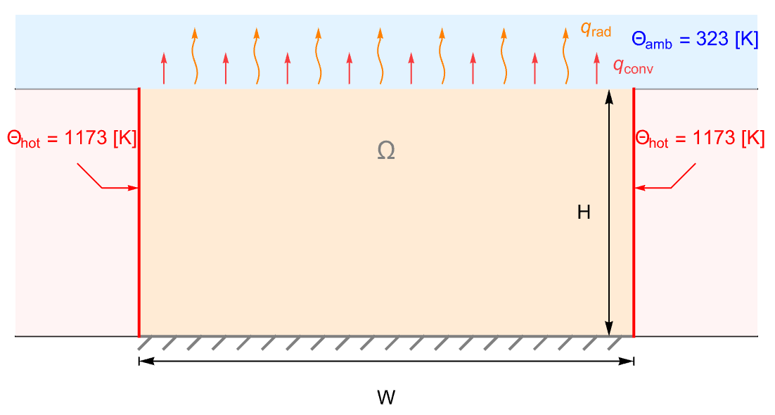
Model a ceramic strip that is embedded in a high-thermal-conductive material. The side boundaries of the strip are maintained at a constant temperature . The top surface of the strip is losing heat via both heat convection and heat radiation to the ambient environment at . The bottom boundary is assumed to be thermally insulated:

Model a temperature field and the thermal radiation and thermal transfer with:

Set up the heat transfer model variables :

Set up a rectangular domain with a width of and a height of :

Specify thermal conductivity :

Set up temperature surface boundary conditions at the left and right boundaries:

Set up a heat transfer boundary condition on the top surface:

Also set up a thermal radiation boundary condition on the top surface:

Set up the equation:

Solve the PDE:

Visualize the solution:

3D (1)

Model a temperature field with two heat conditions at the sides and an orthotropic thermal conductivity :

Set up the heat transfer model variables :

Set up a region :

Specify an orthotropic thermal conductivity :

Specify heat surface conditions:

Set up the equation with a thermal heat flux of applied at the left end for the first 300 seconds:

Solve the PDE:

Visualize the solution:

Time Dependent (1)

Model a temperature field and a thermal heat flux through part of the boundary with:

Set up the heat transfer model variables :

Set up a region :

Specify heat transfer model parameters mass density , specific heat capacity and thermal conductivity :

Specify a thermal heat flux of applied at the left end for the first 300 seconds:

Set up initial conditions:

Set up the equation with a thermal heat flux of applied at the left end for the first 300 seconds:

Solve the PDE:

Visualize the solution:

Time-Dependent Nonlinear (1)

Model a temperature field with a nonlinear heat conductivity term with:

Set up the heat transfer model variables :

Set up a region :

Specify heat transfer model parameters mass density , specific heat capacity and a nonlinear thermal conductivity :

Specify a thermal heat flux of applied at the left end for the first 300 seconds:

Set up initial conditions:

Set up the equation with a thermal heat flux of applied at the left end for the first 300 seconds:

Solve the PDE:

Solve a linear version of the PDE:

Visualize the solutions:

Applications (7)

Boundary Conditions (5)

Compute the temperature field with model variables and parameters with a thermal surface of at the left boundary:

Set up the equation:

Solve the PDE:

Visualize the solution and note the sinusoidal temperature change on the left:

Compute the temperature field with model variables parameters :

Set up the equation with a thermal outflow boundary at the right end:

Define the initial temperature field:

Solve the PDE:

Visualize the solution and note how the energy leaves the domain through the thermal outflow boundary on the right:

Model a temperature field and a thermal radiation boundary with:

Set up the heat transfer model variables :

Set up a region :

Specify heat transfer model parameters mass density , specific heat capacity and thermal conductivity :

Specify boundary condition parameters with a constant ambient temperature of and a surface emissivity of :

Specify the equation:

Set up initial conditions:

Solve the PDE:

Visualize the solution:

Model a temperature field with heat transfer boundary:

Set up the heat transfer model variables :

Set up a region :

Specify heat transfer model parameters mass density , specific heat capacity and thermal conductivity :

Specify boundary condition parameters with an external flow temperature of and a heat transfer coefficient of :

Specify the equation:

Set up initial conditions:

Solve the PDE:

Visualize the solution:

Model a temperature field and a thermal insulation and a thermal heat flux boundary with:

Set up the heat transfer model variables :

Set up a region :

Specify heat transfer model parameters mass density , specific heat capacity and thermal conductivity :

Specify boundary condition parameters for a heat flux of :

Specify the equation:

Set up initial conditions:

Solve the PDE:

Visualize the solution:

Coupled Equations (2)

Solve a coupled heat and mass transport model:

(partialTheta(t, x))/(partialt)+del .(-k del Theta(t,x))-Q^(︷^( heat transfer model )) = 0; (partialc(t,x))/(partialt)+del .(-d del c(t,x))-R^(︷^( mass transport model )) = 0

Set up the heat transfer mass transport model variables :

Set up a region :

Specify heat transfer and mass transport model parameters, heat source , thermal conductivity , mass diffusivity and mass source :

Set up the model and initial conditions:

Set up initial conditions:

Solve the model:

Visualize the solution:

Solve a coupled heat transfer and mass transport model with a thermal transfer value and a mass flux value on the boundary:

(partialTheta(t, x))/(partialt)+del .(-k del Theta(t,x))-Q^(︷^( heat transfer model )) = |_(Gamma_(x=1))h (Theta_(ext)(t,x)-Theta(t,x))^(︷^( heat transfer boundary )); (partialc(t,x))/(partialt)+del .(-d del c(t,x))-R^(︷^( mass transport model )) = |_(Gamma_(x=0||x=1))q (t,x)^(︷^( mass flux boundary ))