ObservableModelQ

系 sys が可観測であればTrueを，それ以外の場合はFalseを与える．

部分系 sub が可観測であればTrueを与える．

詳細とオプション

有限時間におけるからのモデルの軌跡がその近傍からの他の状態の軌跡と識別可能な場合，その状態空間モデルはにおいて可観測であると言われる．
系 sys は標準およびディスクリプタのStateSpaceModelあるいはAffineStateSpaceModelでよい．
次の部分系 sub を指定することができる．

	All	系全体
	"Fast"	速い部分系
	"Slow"	遅い部分系
	"Unstable"	不安定な部分系
	{λ₁,…}	固有モードの部分系

KroneckerModelDecompositionにあるように，"Fast"と"Slow"の部分系が主にディスクリプタ状態空間モデルに適用される．
固有モード λ_iについてはJordanModelDecompositionに記述されている．
ObservableModelQには以下の設定のMethodオプションが使える．

	Automatic	適切な検定を自動的に選ぶ
	"Distribution"	可観測性分布の階数を使う
	"Gramian"	可観測性グラミアンの階数または正定性を使う
	"Matrix"	可観測性行列の階数を使う
	"PBH"	Popov–Belevitch–Hautus階数検定を使う

例題

すべて開くすべて閉じる

例 (2)

可観測系：

Wolfram Language code:

ObservableModelQ[StateSpaceModel[{{{Subscript[a, 1], 0}, {0, Subscript[a, 2]}}, 
  {{1}, {1}}, {{Subscript[c, 1], Subscript[c, 2]}}, {{0}}}, 
 SamplingPeriod -> None, SystemsModelLabels -> None]]

非可観測系（第2状態が可観測ではないため）：

Wolfram Language code:

ObservableModelQ[StateSpaceModel[{{{Subscript[a, 1], 0}, {0, Subscript[a, 2]}}, 
  {{1}, {1}}, {{Subscript[c, 1], 0}}, {{0}}}, SamplingPeriod -> None, 
 SystemsModelLabels -> None]]

スコープ (6)

近似係数を持つ系の可観測性を検定する：

Wolfram Language code:

ObservableModelQ[StateSpaceModel[{{{-2.5368, 0.0606}, {4.0987, -2.4631}}, {{0.1509}, {-0.0951}}, 
  {{5.1481, -2.3431}}, {{0}}}, SamplingPeriod -> None, SystemsModelLabels -> None]]

厳密係数：

Wolfram Language code:

ObservableModelQ[StateSpaceModel[{{{17, -45}, {8, -21}}, {{2}, {1}}, {{-2, 5}}, {{0}}}, SamplingPeriod -> None, 
 SystemsModelLabels -> None]]

記号係数：

Wolfram Language code:

ObservableModelQ[StateSpaceModel[{{{0, 1}, {(-Subscript[α, 1])*Subscript[α, 2], 
    -Subscript[α, 1] - Subscript[α, 2]}}, {{0}, {1}}, 
  {{k, 0}}, {{0}}}, SamplingPeriod -> None, SystemsModelLabels -> None]]

多出力系：

Wolfram Language code:

ObservableModelQ[StateSpaceModel[{{{-1, 0}, {0, -3}}, {{1}, {0}}, {{1, 0}, {0, 1}}, {{0}, {0}}}, 
 SamplingPeriod -> None, SystemsModelLabels -> None]]

離散時間系：

Wolfram Language code:

ObservableModelQ[StateSpaceModel[{{{0, 1}, {-2, -1}}, {{0}, {1}}, {{0.5, 2}}, {{0}}}, SamplingPeriod -> 1, 
 SystemsModelLabels -> None]]

ディスクリプタ系：

Wolfram Language code:

ssm = StateSpaceModel[{{{1, 0, 0}, {0, 1, 0}, {0, 0, 0}}, {{0}, {1}, {1}}, {{-1, -6, 10}}, {{0}}, 
  {{0, 1, 0}, {0, 0, 0}, {0, 0, 1}}}, SamplingPeriod -> None, SystemsModelLabels -> None];

Wolfram Language code: ObservableModelQ[ssm]

可観測性は速いモードと遅い部モード両方が可観測であることと等しい（C可観測性）：

Wolfram Language code: {ObservableModelQ[{ssm, "Slow"}], ObservableModelQ[{ssm, "Fast"}]}

個々の固有モードの可観測性を検定する：

Wolfram Language code:

ssm = StateSpaceModel[{{{-2, 1, 0}, {1, -3, 1}, {0, -1, -2}}, {{-1}, {0}, {0}}, {{1, 1, 1}}, {{0}}}, 
 SamplingPeriod -> None, SystemsModelLabels -> None];

固有モードがあるので，この系は可観測ではない：

Wolfram Language code: modes = Eigenvalues[First[Normal[ssm]]]

Wolfram Language code: Table[{λ, ObservableModelQ[{ssm, λ}]}, {λ, modes}]

これは，第2状態を観測する術がないジョルダン系にも見ることができる：

Wolfram Language code: JordanModelDecomposition[ssm]//Last

AffineStateSpaceModelの可観測性を検定する：

Wolfram Language code:

ObservableModelQ[AffineStateSpaceModel[{{Subscript[x, 1], Subscript[x, 1]^2}, 
  {{Subscript[x, 2]}, {0}}, {Subscript[x, 2]}, {{0}}}, 
 {Subscript[x, 1], Subscript[x, 2]}, Automatic, {Automatic}, Automatic, 
 SamplingPeriod -> None]]

操作点が与えられているなら，における可観測性が検定できる：

Wolfram Language code:

ObservableModelQ[AffineStateSpaceModel[{{Subscript[x, 1]*Subscript[x, 2], 0}, {{0}, {1}}, 
  {Subscript[x, 1]}, {{0}}}, {{Subscript[x, 1], 0}, 
  {Subscript[x, 2], 0}}, Automatic, {Automatic}, Automatic, SamplingPeriod -> None]]

この系は生成点において可観測である：

Wolfram Language code:

ObservableModelQ[AffineStateSpaceModel[{{Subscript[x, 1]*Subscript[x, 2], 0}, {{0}, {1}}, 
  {Subscript[x, 1]}, {{0}}}, {Subscript[x, 1], 
  Subscript[x, 2]}, Automatic, {Automatic}, Automatic, SamplingPeriod -> None]]

オプション (6)

Method (6)

デフォルトで，可観測性行列は厳密系および記号系に用いられる：

Wolfram Language code:

ssm = StateSpaceModel[{{{0, 10}, {1, 0}}, {{0}, {1}}, {{0, 1}}, {{0}}}, SamplingPeriod -> None, 
 SystemsModelLabels -> None];

Wolfram Language code: ObservableModelQ[ssm, Method -> "Matrix"]

ObservabilityMatrixが最大階数であれば，この系は可観測である：

Wolfram Language code: om = ObservabilityMatrix[ssm];

Wolfram Language code: MatrixRank[om]

可観測性グラミアンは安定した数値系に用いられる：

Wolfram Language code:

ssm = StateSpaceModel[{{{0, 1., 0.}, {0, 0., 1.}, {-1., -2., -2.}}, {{0}, {0}, {1.}}, {{1., 0, 0}}, 
  {{0}}}, SamplingPeriod -> None, SystemsModelLabels -> None];

Wolfram Language code: ObservableModelQ[ssm, Method -> "Gramian"]

ObservabilityGramianが最大階数であれば，この系は可観測である：

Wolfram Language code: og = ObservabilityGramian[ssm];

Wolfram Language code: MatrixRank[og]

可観測性グラミアンについては，このことは，これが正定値であることと等しい：

Wolfram Language code: PositiveDefiniteMatrixQ[og]

PBH階数検定は，他のすべての数値系に用いられる：

Wolfram Language code:

ssm = StateSpaceModel[{{{0, 1.}, {1., 0}}, {{0}, {1.}}, {{0.05, 1.}}, {{0}}}, SamplingPeriod -> None, 
 SystemsModelLabels -> None];

Wolfram Language code: ObservableModelQ[ssm, Method -> "PBH"]

がすべてのについて最大階数なので，この系は可観測である：

Wolfram Language code: {a, c} = Normal[ssm][[{1, 3}]];

Wolfram Language code: MatrixRank /@ Table[ArrayFlatten[{{λ IdentityMatrix[2] - a}, {c}}], {λ, Eigenvalues[a]}]

可観測性共分布は，入力線形系に用いられる：

Wolfram Language code:

ObservableModelQ[AffineStateSpaceModel[{{0, Subscript[x, 1]}, {{1 + Subscript[x, 1]}, 
   {0}}}, {Subscript[x, 1], Subscript[x, 2]}, Automatic, 
 {Automatic, Automatic}, Automatic, SamplingPeriod -> None], Method -> "Distribution"]

線形系については，可観測性行列と共分布に基づいた検定は等しい：

Wolfram Language code:

Table[ObservableModelQ[AffineStateSpaceModel[{{-Subscript[x, 1] + Subscript[x, 2], 
   2*Subscript[x, 1] + Subscript[x, 2]}, {{1}, {-1}}, 
  {Subscript[x, 1]}, {{0}}}, {Subscript[x, 1], 
  Subscript[x, 2]}, {Subscript[, 1]}, {Automatic}, Automatic, 
 SamplingPeriod -> None], Method -> m], {m, {"Matrix", "Distribution"}}]

線形系の可観測性は，入力線形系の可観測性を暗示する：

Wolfram Language code:

asys = AffineStateSpaceModel[{{-Subscript[x, 2] + Subscript[x, 1]*
     Subscript[x, 2], -Subscript[x, 1] - 
    Subscript[x, 1]*Subscript[x, 2]}, {{1}, {0}}, 
  {2*Subscript[x, 1]}, {{0}}}, {Subscript[x, 1], 
  Subscript[x, 2]}, Automatic, {Automatic}, Automatic, SamplingPeriod -> None];

Wolfram Language code: lsys = StateSpaceModel[asys];

Wolfram Language code: {ObservableModelQ[lsys], ObservableModelQ[asys]}

入力線形系についての行列検定は，線形化された系について"Matrix"メソッドを用いる：

Wolfram Language code: ObservableModelQ[asys, Method -> "Matrix"]

アプリケーション (2)

の測定から3つの質量すべての位置と速度を推定することができる：

Wolfram Language code:

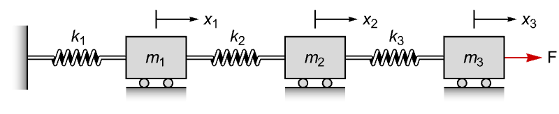
ObservableModelQ[StateSpaceModel[{{{0, 1, 0, 0, 0, 0}, 
   {-(Subscript[k, 1] + Subscript[k, 2])/Subscript[m, 1], 0, 
    Subscript[k, 2]/Subscript[m, 1], 0, 0, 0}, {0, 0, 0, 1, 0, 0}, 
   {Subscript[k, 2]/Subscript[m, 2], 0, 
    -(Subscript[k, 2] + Subscript[k, 3])/Subscript[m, 2], 0, 
    Subscript[k, 3]/Subscript[m, 2], 0}, {0, 0, 0, 0, 0, 1}, 
   {0, 0, Subscript[k, 3]/Subscript[m, 3], 0, 
    -Subscript[k, 3]/Subscript[m, 3], 0}}, 
  {{0}, {0}, {0}, {0}, {0}, {Subscript[m, 3]^(-1)}}, {{1, 0, 0, 0, 0, 0}}, {{0}}}, 
 SamplingPeriod -> None, SystemsModelLabels -> None]]

状態としてのコンデンサー電圧とインダクタ電流，測度としての電流がある電気回路：

Wolfram Language code:

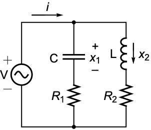
ssm = StateSpaceModel[{{{-𝒞^(-1)/Subscript[R, 1], 0}, 
   {0, (-L^(-1))*Subscript[R, 2]}}, 
  {{1/(𝒞*Subscript[R, 1])}, {L^(-1)}}, 
  {{-Subscript[R, 1]^(-1), 1}}, {{Subscript[R, 1]^(-1)}}}, 
 SamplingPeriod -> None, SystemsModelLabels -> None];

一般に，この系は可観測である：

Wolfram Language code: ObservableModelQ[ssm]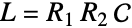

しかし，野場合は可観測ではない：

Wolfram Language code: ObservableModelQ[ssm /. L -> Subscript[R, 1] Subscript[R, 2]𝒞]

特性と関係 (6)

およびを仮定すると，対角系は可観測である：

Wolfram Language code:

ObservableModelQ[StateSpaceModel[{{{Subscript[λ, 1], 0}, {0, Subscript[λ, 2]}}, 
  {{}, {}}, {{Subscript[c, 1], Subscript[c, 2]}}, {{}}}, 
 SamplingPeriod -> None, SystemsModelLabels -> None]]

のとき，最初の状態を観測する方法はない：

Wolfram Language code:

ObservableModelQ[StateSpaceModel[{{{Subscript[λ, 1], 0}, {0, Subscript[λ, 2]}}, 
  {{}, {}}, {{0, Subscript[c, 2]}}, {{}}}, SamplingPeriod -> None, 
 SystemsModelLabels -> None]]

のとき，2番目の状態は直接観測することはできないが，最初の状態を通して間接的に観測することができる：

Wolfram Language code:

ObservableModelQ[StateSpaceModel[{{{Subscript[λ, 1], 1}, {0, Subscript[λ, 2]}}, 
  {{}, {}}, {{Subscript[c, 1], 0}}, {{}}}, SamplingPeriod -> None, 
 SystemsModelLabels -> None]]

のとき，最初の状態は，直接観測することmp2番目の状態から間接的に観測することもできない：

Wolfram Language code:

ObservableModelQ[StateSpaceModel[{{{Subscript[λ, 1], 1}, {0, Subscript[λ, 2]}}, 
  {{}, {}}, {{0, Subscript[c, 2]}}, {{}}}, SamplingPeriod -> None, 
 SystemsModelLabels -> None]]

JordanModelDecompositionで，上記の標準状態空間表現を計算する：

Wolfram Language code:

ssm = StateSpaceModel[{{{0, 1}, {-6, -5}}, {{0}, {1}}, {{5, 1}}, {{0}}}, SamplingPeriod -> None, 
 SystemsModelLabels -> None];

Wolfram Language code: JordanModelDecomposition[ssm]//Last

"PBH"検定を使って各モードのか観測性を計算する：

Wolfram Language code: Table[{λ, ObservableModelQ[{ssm, λ}]}, {λ, {-3, -2}}]

ディスクリプタ系については，KroneckerModelDecompositionは対角系形の一般化である：

Wolfram Language code:

kssm = Last[KroneckerModelDecomposition[ssm = StateSpaceModel[{{{-5, -1, -3}, {-3, 1, -3}, {-6, -2, -2}}, {{2}, {1}, {2}}, {{1, 1, 1}}, {{0}}, 
  {{3, 1, 2}, {4, 0, 2}, {1, 1, 1}}}, SamplingPeriod -> None, SystemsModelLabels -> None]]]

遅い部分系の可観測性をその構造から調べる：

Wolfram Language code: SystemsModelExtract[kssm, All, All, {1, 2}]

もとの系を使ってこれを計算する：

Wolfram Language code: ObservableModelQ[{ssm, "Slow"}]

速い部分系の可観測性をの構造から調べる：

Wolfram Language code: SystemsModelExtract[kssm, All, All, {3}]

もとの系を使ってこれを計算する：

Wolfram Language code: ObservableModelQ[{ssm, "Fast"}]

StateSpaceModelのディスクリプタ行列が最大階数であれば，速い部分系は存在しない：

Wolfram Language code:

ssm = StateSpaceModel[{{{-2, -2}, {8, 12}}, {{1}, {2}}, {{1, 1}}, {{0}}, {{1, 1}, {2, 3}}}, 
 SamplingPeriod -> None, SystemsModelLabels -> None];

したがって，系の完全な可制御性は遅い部分系から評価できる：

Wolfram Language code: {ControllableModelQ[ssm], ControllableModelQ[{ssm, All}], ControllableModelQ[{ssm, "Slow"}]}

AffineStateSpaceModelについては，入力ベクトルの非線形性が可観測性を助ける：

Wolfram Language code:

ObservableModelQ[AffineStateSpaceModel[{{Subscript[x, 2], Subscript[x, 3], 0}, 
  {{0}, {Subscript[x, 1]}, {0}}, {Subscript[x, 2]}, {{0}}}, 
 {Subscript[x, 1], Subscript[x, 2], Subscript[x, 3]}, 
 Automatic, {Automatic}, Automatic, SamplingPeriod -> None]]

線形入力ベクトルのある系は可観測ではない：

Wolfram Language code:

ObservableModelQ[AffineStateSpaceModel[{{Subscript[x, 2], Subscript[x, 3], 0}, 
  {{0}, {α}, {0}}, {Subscript[x, 2]}, {{0}}}, 
 {Subscript[x, 1], Subscript[x, 2], Subscript[x, 3]}, 
 Automatic, {Automatic}, Automatic, SamplingPeriod -> None]]

可観測ではない系は，区別できない初期状態を持つ：

Wolfram Language code:

assm = AffineStateSpaceModel[{{Subscript[x, 1]*Subscript[x, 2], 0}, {{0}, {1}}, 
  {Subscript[x, 1]}, {{0}}}, {{Subscript[x, 1], 0}, 
  {Subscript[x, 2], 0}}, Automatic, {Automatic}, Automatic, SamplingPeriod -> None];

Wolfram Language code: ObservableModelQ[assm]

およびの2つの初期状態は，区別できない出力を生成する：

Wolfram Language code:

Table[OutputResponse[{assm, ic}, 1, {t, 0, 5}], {ic, {{0, 0}, {0, 0.5}}}];
Plot[%, {t, 0, 5}]

考えられる問題 (1)

漸近的に安定ではない系についてはグラミアンメソッドは信頼できない：

Wolfram Language code:

ssm = StateSpaceModel[{{{12, 15, 13}, {-10, -13, -10}, {0, 0, -1}}, {{10/3}, {-2}, {2/3}}, 
  {{3/2, 5/2, 3}}, {{0}}}, SamplingPeriod -> None, SystemsModelLabels -> None];
Table[ObservableModelQ[ssm, Method -> m], {m, {"Gramian", "Matrix", "PBH"}}]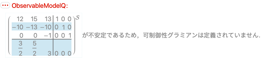

Wolfram Language code: Eigenvalues@First@Normal@ssm

Top

その他のラーニングリソース

テクニカルサポート

データサイエンス，金融，ビジネス

工学

科学とテクノロジー

教育のためのテクノロジー

教育イニシアチブ

使い始める

Grow Your Skills

Wolframと繋がる

大人用の教育プログラム

若者のための教育プログラム

読む

ObservableModelQ

詳細とオプション

例題

例 (2)

スコープ (6)

オプション (6)

Method (6)

アプリケーション (2)

特性と関係 (6)

考えられる問題 (1)

テキスト

CMS

APA

BibTeX

BibLaTeX

ObservableModelQ

詳細とオプション

例題

例 (2)

スコープ (6)

オプション (6)

Method (6)

アプリケーション (2)

特性と関係 (6)

考えられる問題 (1)

関連項目

関連するガイド

履歴

テキスト

CMS

APA

BibTeX

BibLaTeX