

SingularValueList
给出一个矩阵 m 的非零奇异值列表.
SingularValueList[{m,a}]
给出 m 关于 a 的广义奇异值.
SingularValueList[m,k]
给出 m 的 k 个最大的奇异值.
SingularValueList[{m,a},k]
给出 m 的 k 个最大的广义奇异值.
更多信息和选项
- 奇异值从最大到最小排序.
- 奇异值的多样性导致了奇异值的重复.
- 在默认情况下,当奇异值大于10-p 的100倍时,它们会保留,其中p 是 Precision[m].
- SingularValueList[m,Tolerance->t] 只有当大于至少 t 倍的最大奇异值时才保留.
- SingularValueList[m,Tolerance->0] 返回所有的奇异值.
- m 可以是矩形矩阵;全部奇异值的数目通常是 Min[Dimensions[m]].
- 可以使用默认零误差的精确符号矩阵.
- 奇异值可以从 Sqrt[Eigenvalues[ConjugateTranspose[m].m]] 获得.
范例
打开所有单元 关闭所有单元基本范例 (2)
SingularValueList[(|   |   |
| - | - |
| 1 | 2 |
| 3 | 4 |)]SingularValueList[(| | | |
| - | - | - |
| 1 | 2 | 3 |
| 4 | 5 | 6 |
| 7 | 8 | 9 |)]MatrixRank[(| | | |
| - | - | - |
| 1 | 2 | 3 |
| 4 | 5 | 6 |
| 7 | 8 | 9 |)]范围 (19)
基本用法 (7)
SingularValueList[(| | | |
| --- | --- | --- |
| 1.1 | 1.3 | 2.1 |
| 2.2 | 2.2 | 3.3 |
| 3.3 | -3 | 4.7 |)]SingularValueList[(| | |
| ----------- | ----------- |
| 0.5 + 0.5 I | 1.1 |
| -I | 3.2 - 4.5 I |)]SingularValueList[{{1, 2}, {3, 4}}]SingularValueList[MatrixExp[RandomReal[1, {2, 2}, WorkingPrecision -> 20]]]FullSimplify[SingularValueList[(| | |
| - | - |
| a | b |
| c | d |)], {a, b, c, d}∈ℝ]m = RandomReal[{1, 9}, {1000, 1000}];AbsoluteTiming[SingularValueList[m];]SingularValueList[(| | | | |
| - | - | -- | - |
| 3 | 2 | 2 | 7 |
| 9 | 3 | -2 | 1 |)]奇异值的子集 (5)
m = (| | | | | |
| --- | --- | ---- | ----- | ------ |
| 0.5 | 0.5 | 0.5 | 0 | 0 |
| 1. | 2. | 4. | 8. | 0 |
| 1.5 | 4.5 | 13.5 | 40.5 | 121.5 |
| 0 | 8. | 32. | 128. | 512. |
| 0 | 0 | 62.5 | 312.5 | 1562.5 |);
SingularValueList[m, 3]SingularValueList[m, -3]求四个最大的奇异值,包括零值,或者尽可能多的奇异值(如果数量不够的话):
SingularValueList[(| | | |
| --- | --- | --- |
| 0.5 | 1. | 1.5 |
| 2. | 2.5 | 3. |
| 3.5 | 4. | 4.5 |), UpTo[4]]SingularValueList[(| | | |
| --- | --- | --- |
| 0.5 | 1. | 1.5 |
| 2. | 2.5 | 3. |
| 3.5 | 4. | 4.5 |), -2]SingularValueList[{{2, 0, 0}, {0, 2, 0}, {0, 0, 2}}]mat = {{(7/2), 0, (1/2), 0}, {0, 3, 0, 1}, {(1/2), 0, (7/2), 0}, {0, 1, 0, 3}};SingularValueList[mat]SingularValueList[mat, 3]SingularValueList[mat, -3]广义奇异值 (3)
m = {{1.5, 1.3}, {3.1, 2.2}};
a = {{1.1, 5.1}, {4.2, 3.4}};
SingularValueList[{m, a}]a = (| | | |
| --- | --- | --- |
| 1. | 1.5 | 2. |
| 3.1 | 2. | 2.9 |
| 3. | 2. | 1. |);b = (| | | |
| --- | --- | --- |
| 1.3 | 0.5 | 1.1 |
| 0. | 1.5 | 2.3 |
| 1. | 0. | 1. |);SingularValueList[{a, b}, -2]m = (| | |
| ---------------------------------------- | ---------------------------------------- |
| 4.641175490606916 + 7.207263282382337 I | 2.522671922520866 + 8.989217121399136 I |
| 4.114478069008367 + 7.010706036954508 I | 8.95961276370625 + 3.569738897382109 I |
| 4.405169936758572 + 4.4509297530197465 I | 9.145107926643146 + 6.3767022076415465 I |);a = (| | |
| --------------------------------------- | ---------------------------------------- |
| 7.341517476299638 + 9.810565178638917 I | 8.24181899398409 + 3.4570598473462972 I |
| 7.775955216608212 + 1.68269060515731 I | 3.944961113408187 + 1.4889990223210265 I |
| 6.431377195364613 + 6.245150387114993 I | 7.026661544586792 + 1.0790173484547747 I |);SingularValueList[{m, a}]特殊矩阵 (4)
SparseArray[{{1, 3} -> 2, {2, 2} -> 3, {3, 1} -> 1, {4, 2} -> 5}, {4, 4}]SingularValueList[%]SparseArray[{{x_, y_} /; Abs[x - y] < 3 -> 1}, {150, 150}]SingularValueList[%, 3]//FullSimplifySymmetrizedArray[{{1, 1} -> 2, {1, 2} -> 1}, {2, 2}, Symmetric[All]]SingularValueList[%]QuantityArray[{{1, 2}, {3, 4}}, {"Meters", "Meters"}]SingularValueList[%]IdentityMatrix 总有全为 1 的奇异值:
SingularValueList[IdentityMatrix[12]]HilbertMatrix 的奇异值:
SingularValueList[HilbertMatrix[5]]//FullSimplify选项 (2)
Tolerance (2)

m = N[HilbertMatrix[10]];{Subscript[σ, 1]} = SingularValueList[m, 1];Select[SingularValueList[m], # > 0.1 Subscript[σ, 1]&]设置 Tolerance 为  ,将直接计算奇异值的相同集:
SingularValueList[m, Tolerance -> 0.1]m = HilbertMatrix[16];Length[SingularValueList[m]]Length[SingularValueList[N[m]]]SingularValueList[N[m], Tolerance -> 0]N[SingularValueList[m]]应用 (4)


m = (| | | |
| ------------------- | ------------------- | ------------------ |
| 0.6201924059167849 | 0.1642012623471385 | 0.9488900631268065 |
| 0.45081828391187817 | 0.23528005253744255 | 0.5556683503523119 |
| 0.6490685022331557 | 0.8994304255663148 | 0.4108954380673717 |);
SingularValueList[m, 1]//First使用 MaxValue 验证结果:
MaxValue[(Norm[m.x]/Norm[x]), x∈Vectors[3, Reals]]


m = (| | | |
| ------------------ | ------------------ | ------------------- |
| 0.61 | 0.6596700568069829 | 0.21806383036829602 |
| 0.9065034103282616 | 0.32 | 0.39008198633165536 |
| 0.9749976665586482 | 0.5298619922699106 | 0.7332553638224806 |);因为矩阵的行数至少与列数一样多,所以最小值是  的最小奇异值:
SingularValueList[m, -1]//First使用 MinValue 验证结果:
MinValue[Norm[m.x], x∈Sphere[]]矩阵的算子范数,也称为谱范数或二范数,定义为 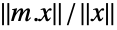 的最大值,其中约束条件为
 . 求以下
 的算子范数:
m = (|   |   |   |   |
| - | - | - | - |
| 1 | 2 | 3 | 4 |
| 5 | 6 | 7 | 8 |);

SingularValueList[m, 1]//First使用 Norm 验证结果:
% == Norm[m]


m = (| | | | | |
| ------------------- | ------------------ | ------------------- | ------------------- | ------------------- |
| 0.5586541141266836 | 0.4836196860997566 | 0.43001371472761707 | 0.15584341399194623 | 0.5776446005074791 |
| 0.03069348146554618 | 0.5690912070366865 | 0.9683326899888793 | 0.580 | 0.5052068378482946 |
| 0.6553340778639707 | 0.3059598694903798 | 0.3931179458877401 | 0.5208999887331609 | 0.27321537200542423 |
| 0.03595071365286251 | 0.9210532614194069 | 0.9985000839819722 | 0.41170277644341935 | 0.3839108065740755 |
| 0.5809025186735828 | 0.6117636142636071 | 0.11827188288474355 | 0.31845314947311976 | 0.35583919578557843 |);
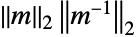
sv = SingularValueList[m]sv[[1]] == Norm[m, 2](1/sv[[-1]])使用 Norm 进行验证:
% == Norm[Inverse[m], 2]

sv[[1]] / sv[[-1]]属性和关系 (11)


m = RandomInteger[{0, 9}, {7, 5}];SingularValueList[m] == DeleteCases[Sqrt[Eigenvalues[m.ConjugateTranspose[m]]], 0]//FullSimplify
SingularValueList[m] == DeleteCases[Sqrt[Eigenvalues[ConjugateTranspose[m].m]], 0]//FullSimplify


m = (| | | |
| - | -- | -- |
| 1 | 0 | 1 |
| 0 | 1 | -1 |
| 1 | 1 | 0 |
| 1 | -1 | 2 |);SingularValueList[m, Tolerance -> 0]
% == Sqrt[Eigenvalues[ConjugateTranspose[m].m]]Sqrt[Eigenvalues[m.ConjugateTranspose[m]]]m 和 ConjugateTranspose[m] 有相同的奇异值:
m = RandomComplex[1 + I, {5, 7}];
SingularValueList[m] == SingularValueList[ConjugateTranspose[m]]m = RandomInteger[9, {5, 5}];
Abs[Det[m]] == Times@@SingularValueList[m, Tolerance -> 0]//FullSimplify对于正规矩阵 n,奇异值等于 Abs[Eigenvalues[n]]:
m = {{1, 2, -1}, {-1, 1, 2}, {2, -1, 1}};
NormalMatrixQ[m]SingularValueList[m] == Abs[Eigenvalues[m]]MatrixRank[m] 等于非零奇异值的数量:
m = RandomInteger[1, {6, 6}];
MatrixRank[m] == Length[SingularValueList[m]]

m = RandomReal[1, {5, 5}];
SingularValueList[Inverse[m]] == Reverse[(1/SingularValueList[m])]
对于 m 的子矩阵 s,m 的最大奇异值大于或等于 s 的奇异值:
m = RandomReal[1, {5, 5}];
s = m[[RandomSample[Range[5], 3], RandomSample[Range[5], 4]]];First[SingularValueList[m, 1]] ≥ First[SingularValueList[s, 1]]


m = RandomComplex[1 + I, {3, 3}];
a = RandomComplex[1 + I, {3, 3}];SingularValueList[{m, a}] == Sqrt[Eigenvalues[{ConjugateTranspose[m].m, ConjugateTranspose[a].a}]]

SingularValueList[{m, a}] == Sqrt[Eigenvalues[{m.ConjugateTranspose[m], a.ConjugateTranspose[a]}]]


m = (| | | |
| ---- | ---- | ---- |
| 0.2 | 0.05 | 0.91 |
| 0.25 | 0.83 | 0.21 |
| 0.2 | 0.73 | 0.43 |);a = (| | | |
| ------------------ | ---- | ---- |
| 0.01 | 0.28 | 0.63 |
| 0.5700000000000001 | 0.25 | 0.63 |
| 0.8 | 0.19 | 0.13 |);SingularValueList[{m, a}]MaxValue[(Norm[m.x]/Norm[a.x]), x∈Sphere[]]
v1 = ArgMax[(Norm[m.x]/Norm[a.x]), x∈Sphere[]];


MaxValue[{(Norm[m.x]/Norm[a.x]), x.a.a.v1 == 0}, x∈Sphere[]]通过要求  与所有前面的输入
 -正交,可以找到每个后续奇异值:
v2 = ArgMax[{(Norm[m.x]/Norm[a.x]), x.a.a.v1 == 0}, x∈Sphere[]];MaxValue[{(Norm[m.x]/Norm[a.x]), x.a.a.v1 == 0 && x.a.a.v2 == 0}, x∈Sphere[]]


m = RandomComplex[1 + I, {3, 3}];
a = RandomComplex[1 + I, {3, 3}];
SingularValueList[{m, a}] == SingularValueList[{ConjugateTranspose[m], ConjugateTranspose[a]}]
文本
Wolfram Research (2003),SingularValueList,Wolfram 语言函数,https://reference.wolfram.com/language/ref/SingularValueList.html (更新于 2015 年).
CMS
Wolfram 语言. 2003. "SingularValueList." Wolfram 语言与系统参考资料中心. Wolfram Research. 最新版本 2015. https://reference.wolfram.com/language/ref/SingularValueList.html.
APA
Wolfram 语言. (2003). SingularValueList. Wolfram 语言与系统参考资料中心. 追溯自 https://reference.wolfram.com/language/ref/SingularValueList.html 年