

StateOutputEstimator
StateOutputEstimator[ssm,l]
构建 StateSpaceModel ssm 的估值器,估值器增益矩阵为 l.
StateOutputEstimator[{ssm,sensors},l]
只将 sensors 作为 ssm 的测量使用.
StateOutputEstimator[{ssm,sensors,dinputs},l]
将 dinputs 指定为 ssm 的确定性输入.
更多信息和选项
- 标准状态空间模型 ssm 可以以 StateSpaceModel[{a,b,c,d}] 给出,其中 a、b、c 和 d 表示连续时间或者离散时间系统中的状态、输入、输出和传递矩阵:
-

连续时间系统 
离散时间系统 - 在连续时间或者离散时间下,描述器状态空间模型 ssm 可以按 StateSpaceModel[{a,b,c,d,e}] 给出:
-

连续时间系统 
离散时间系统 - StateOutputEstimator 也接受由 AffineStateSpaceModel 和 NonlinearStateSpaceModel 指定的非线性系统.
- 对非线性系统,当构建估值器时要考虑状态的动作值和输入变量.
- 输入
 可以包括随机输入
 和确定性输入
 .
- 参数 dinputs 是整数列表,指定
 中
 的位置.
- 输出
 可以包括测量
 和其他输出.
- 参数 sensors 是整数列表,指定
 中
 的位置.
- StateOutputEstimator[ssm,l] 等价于 StateOutputEstimator[{ssm,All,All},l].
- 估值器增益 l 可以使用 EstimatorGains、LQEstimatorGains 或者 DiscreteLQEstimatorGains 计算.
- StateOutputEstimator[ssm,LQEstimatorGains[ssm,…],…] 给出 Kalman 估值器.
- StateOutputEstimator[ssm,EstimatorGains[ssm,…],…] 给出 Luenberger 估值器.
- StateOutputEstimator 支持 Method 选项. 可以给出下列显式设置:
-
"CurrentEstimator" 构建当前估值器 "PredictionEstimator" 构建预测估值器 - 当前估计基于到目前时刻的测量.
- 预测估计基于到前一时刻的测量.
- 对于连续时间系统,StateOutputEstimator 给出具有动态的估值器
 . 下标为
 和
 的矩阵是与确定性输入
 和感应器
 相关联的子矩阵.
- 离散时间系统的预测估值器具有动态
 .
- 对于离散时间系统,StateOutputEstimator[…,Method->"CurrentEstimator"] 给出具有动态的估值器
 ,而当前状态估计
 从当前测量
 得到,为
 .
- 对于离散系统,预测增益
 与当前增益
 之间的关系为
 .
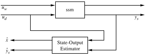
- 具有估值器的系统的方框图:
- 估值器模型的输入是确定性输入
 和测量
 .
- 估值器模型的输出包括估计状态
 和测量
 的估计.
范例
打开所有单元 关闭所有单元基本范例 (3)
StateOutputEstimator[StateSpaceModel[{{{-2}}, {{0.6, 0.4}}, {{0.5}, {-0.4}}, {{1, -1}, {0, 1}}}, SamplingPeriod -> None,
SystemsModelLabels -> None], (-0.67 -0.33)]StateOutputEstimator[{StateSpaceModel[{{{a}}, {{Subscript[b, 1],
Subscript[b, 2]}}, {{Subscript[c, 1]},
{Subscript[c, 2]}}, {{Subscript[d, 11],
Subscript[d, 12]}, {Subscript[d, 21],
Subscript[d, 22]}}}, SamplingPeriod -> None, SystemsModelLabels -> None], 2}, (1)]对于离散时间系统,StateOutputEstimator 组成一个离散时间估值器:
StateOutputEstimator[{StateSpaceModel[{{{a}}, {{Subscript[b, 1],
Subscript[b, 2]}}, {{Subscript[c, 1]},
{Subscript[c, 2]}}, {{Subscript[d, 11],
Subscript[d, 12]}, {Subscript[d, 21],
Subscript[d, 22]}}}, SamplingPeriod -> τ, SystemsModelLabels -> None], 1}, (1)]范围 (8)
StateOutputEstimator[StateSpaceModel[{{{a}}, {{b}}, {{c}}, {{d}}},
SamplingPeriod -> None, SystemsModelLabels -> None], (L)]StateOutputEstimator[{StateSpaceModel[{{{a}}, {{b}}, {{c}}, {{d}}},
SamplingPeriod -> None, SystemsModelLabels -> None], All, None}, (L)]系统的估值器,其中所有输出都被测量,并且所有输入都是确定性的:
StateOutputEstimator[StateSpaceModel[{{{a}}, {{Subscript[b, 1],
    Subscript[b, 2]}}, {{Subscript[c, 1]},
   {Subscript[c, 2]}}, {{Subscript[d, 11],
    Subscript[d, 12]}, {Subscript[d, 21],
Subscript[d, 22]}}}, SamplingPeriod -> None, SystemsModelLabels -> None], (Subscript[L, 1] Subscript[L, 2])]StateOutputEstimator[{StateSpaceModel[{{{a}}, {{Subscript[b, 1],
Subscript[b, 2]}}, {{Subscript[c, 1]},
{Subscript[c, 2]}}, {{Subscript[d, 11],
Subscript[d, 12]}, {Subscript[d, 21],
Subscript[d, 22]}}}, SamplingPeriod -> None, SystemsModelLabels -> None], 1}, (Subscript[L, 1])]StateOutputEstimator[{StateSpaceModel[{{{a}}, {{Subscript[b, 1],
Subscript[b, 2]}}, {{Subscript[c, 1]},
{Subscript[c, 2]}}, {{Subscript[d, 11],
Subscript[d, 12]}, {Subscript[d, 21],
Subscript[d, 22]}}}, SamplingPeriod -> None, SystemsModelLabels -> None], 1, 1}, (Subscript[L, 1])]StateOutputEstimator[{StateSpaceModel[{{{a}}, {{Subscript[b, 1],
Subscript[b, 2]}}, {{Subscript[c, 1]},
{Subscript[c, 2]}}, {{Subscript[d, 11],
Subscript[d, 12]}, {Subscript[d, 21],
Subscript[d, 22]}}}, SamplingPeriod -> None, SystemsModelLabels -> None], All, None}, (Subscript[L, 1] Subscript[L, 2])]StateOutputEstimator[StateSpaceModel[{{{a}}, {{Subscript[b, 1],
Subscript[b, 2]}}, {{Subscript[c, 1]},
{Subscript[c, 2]}}, {{Subscript[d, 1], 0},
{0, Subscript[d, 2]}}, {{e}}}, SamplingPeriod -> None,
SystemsModelLabels -> None], (Subscript[l, 1] Subscript[l, 2])]一个对 AffineStateSpaceModel 的估值器:
asys = AffineStateSpaceModel[{{-Sin[0.5 - Subscript[x, 1]],
   Subscript[x, 1] - Subscript[x, 2]}, {{1}, {0}},
  {Subscript[x, 1]}, {{0}}}, {{Subscript[x, 1], 0.5},
  {Subscript[x, 2], 0}}, {u}, {Automatic}, Automatic,
SamplingPeriod -> None];ℓ = EstimatorGains[asys, {-1, -2}]estim = StateOutputEstimator[asys, ℓ]Subscript[y, a] = OutputResponse[{asys, {-3, 0}}, Sin[t], {t, 0, 25}];Subscript[y, e] = OutputResponse[estim, Join[{Sin[t]}, Subscript[y, a]], {t, 0, 25}][[-1]];Plot[{Subscript[y, a], Subscript[y, e]}, {t, 0, 4}, PlotLegends -> {"actual", "estimated"}, PlotRange -> All]选项 (2)
Method (2)
ssm = StateSpaceModel[{{{a}}, {{Subscript[b, 1],
    Subscript[b, 2]}}, {{Subscript[c, 1]},
   {Subscript[c, 2]}}, {{Subscript[d, 11],
    Subscript[d, 12]}, {Subscript[d, 21],
Subscript[d, 22]}}}, SamplingPeriod -> τ, SystemsModelLabels -> None];gains = (Subscript[g, 1] Subscript[g, 2]);StateOutputEstimator[ssm, gains]StateOutputEstimator[ssm, gains, Method -> "PredictionEstimator"]Table[StateOutputEstimator[StateSpaceModel[{{{a}}, {{Subscript[b, 1],
Subscript[b, 2]}}, {{Subscript[c, 1]},
{Subscript[c, 2]}}, {{Subscript[d, 11],
Subscript[d, 12]}, {Subscript[d, 21],
Subscript[d, 22]}}}, SamplingPeriod -> None, SystemsModelLabels -> None], (Subscript[g, 1] Subscript[g, 2]), Method -> m], {m, {"CurrentEstimator", "PredictionEstimator"}}]Equal@@%应用 (1)
ssm = StateSpaceModel[{{{-1, 0, 0}, {0, -2, 0}, {0, 0, -3}}, {{-1}, {0}, {1}},
{{1, -1, 0}, {1.5, 0, -1}}, {{1}, {0}}}, SamplingPeriod -> None, SystemsModelLabels -> None];l = EstimatorGains[ssm, {-3 + 4I , -3 - 4I , -12}];obsv = StateOutputEstimator[ssm, l];ic = RandomReal[2, 3];x = StateResponse[{ssm, ic}, E^-t, {t, 5}];y = OutputResponse[{ssm, ic}, E^-t, {t, 5}];xhat = OutputResponse[SystemsModelExtract[obsv, All, {1, 2, 3}], Join[{E^-t}, y], {t, 5}];Grid[{MapIndexed[Plot[#, {t, 0, 5}, PlotLabel -> "State " <> ToString[First[#2]], PlotRange -> All, PlotStyle -> {Automatic, Dashed}]&, Thread[{x, xhat}]]}]yhat = OutputResponse[SystemsModelExtract[obsv, All, {4, 5}], Join[{E^-t}, y], {t, 5}];MapIndexed[Plot[#, {t, 0, 5}, PlotLabel -> "Output " <> ToString[First[#2]], PlotRange -> All, PlotStyle -> {Automatic, Dashed}]&, Thread[{y, yhat}]]属性和关系 (2)
StateOutputEstimator 估计系统的状态和输出:
ssm = StateSpaceModel[{{{0.2, 0}, {0, 0.5}}, {{0.1, 0}, {-1, -0.5}}, {{0.001, 0.001}}, {{0, 0}}},
SamplingPeriod -> 0.1, SystemsModelLabels -> None];l = EstimatorGains[ssm, {0.1, 0.4}];est = StateOutputEstimator[ssm, l]SystemsModelExtract[est, All, {1, 2}]SystemsModelExtract[est, All, {3}]ssm = StateSpaceModel[{{{0, 1}, {-1, 2}}, {{0, 0}, {1, 1}}, {{0.005, 0.003}}, {{0, 0}}},
SamplingPeriod -> 0.1, SystemsModelLabels -> None];l = LQEstimatorGains[{ssm, All, 1}, {(0.001), (0.1)}];kest = StateOutputEstimator[{ssm, All, 1}, l]直接使用 KalmanEstimator:
KalmanEstimator[{ssm, All, 1}, {(0.001), (0.1)}]文本
Wolfram Research (2010),StateOutputEstimator,Wolfram 语言函数,https://reference.wolfram.com/language/ref/StateOutputEstimator.html (更新于 2014 年).
CMS
Wolfram 语言. 2010. "StateOutputEstimator." Wolfram 语言与系统参考资料中心. Wolfram Research. 最新版本 2014. https://reference.wolfram.com/language/ref/StateOutputEstimator.html.
APA
Wolfram 语言. (2010). StateOutputEstimator. Wolfram 语言与系统参考资料中心. 追溯自 https://reference.wolfram.com/language/ref/StateOutputEstimator.html 年