"Extrapolation" Method for NDSolve
Introduction
Extrapolation methods are a class of arbitrary-order methods with automatic order and step-size control. The error estimate comes from computing a solution over an interval using the same method with a varying number of steps and using extrapolation on the polynomial that fits through the computed solutions, giving a composite higher-order method [BS64]. At the same time, the polynomials give a means of error estimation.
Typically, for low precision, the extrapolation methods have not been competitive with Runge–Kutta-type methods. For high precision, however, the arbitrary order means that they can be arbitrarily faster than fixed-order methods for very precise tolerances.
The order and step-size control are based on the codes odex.f and seulex.f described in [HNW93] and [HW96].
Needs["DifferentialEquations`NDSolveProblems`"];
Needs["DifferentialEquations`NDSolveUtilities`"];
"Extrapolation"
The method "DoubleStep" performs a single application of Richardson's extrapolation for any one-step integration method and is described within "DoubleStep Method for NDSolve".
"Extrapolation" generalizes the idea of Richardson's extrapolation to a sequence of refinements.
Consider a differential system
Let ![]() be a basic step size; choose a monotonically increasing sequence of positive integers
be a basic step size; choose a monotonically increasing sequence of positive integers
and define the corresponding step sizes
Choose a numerical method of order ![]() and compute the solution of the initial value problem by carrying out
and compute the solution of the initial value problem by carrying out ![]() steps with step size
steps with step size ![]() to obtain
to obtain
Extrapolation is performed using the Aitken–Neville algorithm by building up a table of values,
where ![]() is either 1 or 2 depending on whether the base method is symmetric under extrapolation.
is either 1 or 2 depending on whether the base method is symmetric under extrapolation.
A dependency graph of the values in (1) illustrates the relationship.
Considering ![]() ,
, ![]() ,
, ![]() is equivalent to Richardson's extrapolation.
is equivalent to Richardson's extrapolation.
For non-stiff problems the order of ![]() in (2) is
in (2) is ![]() . For stiff problems the analysis is more complicated and involves the investigation of perturbation terms that arise in singular perturbation problems [HNW93, HW96].
. For stiff problems the analysis is more complicated and involves the investigation of perturbation terms that arise in singular perturbation problems [HNW93, HW96].
Extrapolation Sequences
Any extrapolation sequence can be specified in the implementation. Some common choices are as follows.
NDSolve`RombergSequenceFunction[1, 10]NDSolve`BulirschSequenceFunction[1, 10]NDSolve`HarmonicSequenceFunction[1, 10]A sequence that satisfies ![]() has the effect of minimizing the roundoff errors for an order-
has the effect of minimizing the roundoff errors for an order-![]() base integration method.
base integration method.
NDSolve`OptimalRoundingSequenceFunction[1, 10, 2]Default[myseqfun, 3] = 1;
myseqfun[n1_, n2_, p_.] := Range[n1, n2]The sequence with lowest cost is the harmonic sequence, but this is not without problems since rounding errors are not damped.
Rounding Error Accumulation
For high-order extrapolation an important consideration is the accumulation of rounding errors in the Aitken–Neville algorithm (3).
As an example consider Exercise 5 of Section II.9 in [HNW93].
Suppose that the entries ![]() are disturbed with rounding errors
are disturbed with rounding errors ![]() and compute the propagation of these errors into the extrapolation table.
and compute the propagation of these errors into the extrapolation table.
Due to the linearity of the extrapolation process (4), suppose that the ![]() are equal to zero and take
are equal to zero and take ![]() .
.
This shows the evolution of the Aitken–Neville algorithm (5) on the initial data using the harmonic sequence and a symmetric order-two base integration method, ![]() .
.
Hence, for an order-sixteen method approximately two decimal digits are lost due to rounding error accumulation.
This model is somewhat crude because, as you will see in "Rounding Error Reduction", it is more likely that rounding errors are made in ![]() than in
than in ![]() for
for ![]() .
.
Rounding Error Reduction
It seems worthwhile to look for approaches that can reduce the effect of rounding errors in high-order extrapolation.
Selecting a different step sequence to diminish rounding errors is one approach, although the drawback is that the number of integration steps needed to form the ![]() in the first column of the extrapolation table requires more work.
in the first column of the extrapolation table requires more work.
Some codes, such as STEP, take active measures to reduce the effect of rounding errors for stringent tolerances [SG75].
An alternative strategy, which does not appear to have received a great deal of attention in the context of extrapolation, is to modify the base-integration method in order to reduce the magnitude of the rounding errors in floating-point operations. This approach, based on ideas that dated back to [G51], and used to good effect for the two-body problem in [F96b] (for background see also [K65], [M65a], [M65b], [V79]), is explained next.
Base Methods
The following methods are the most common choices for base integrators in extrapolation.
For efficiency, these have been built into NDSolve and can be called via the Method option as individual methods.
The implementation of these methods has a special interpretation for multiple substeps within "DoubleStep" and "Extrapolation".
The NDSolve framework for one-step methods uses a formulation that returns the increment or update to the solution. This is advantageous for geometric numerical integration where numerical errors are not damped over long time integrations. It also allows the application of efficient correction strategies such as compensated summation. This formulation is also useful in the context of extrapolation.
The methods are now described together with the increment reformulation that is used to reduce rounding error accumulation.
Multiple Euler Steps
Given ![]() ,
, ![]() , and
, and ![]() , consider a succession of
, consider a succession of ![]() integration steps with step size
integration steps with step size ![]() carried out using Euler's method:
carried out using Euler's method:
Correspondence with Explicit Runge–Kutta Methods
It is well-known that, for certain base integration schemes, the entries ![]() in the extrapolation table produced from (9) correspond to explicit Runge–Kutta methods (see Exercise 1, Section II.9 in [HNW93]).
in the extrapolation table produced from (9) correspond to explicit Runge–Kutta methods (see Exercise 1, Section II.9 in [HNW93]).
For example, (10) is equivalent to an ![]() -stage explicit Runge–Kutta method:
-stage explicit Runge–Kutta method:
where the coefficients are represented by the Butcher table:
Reformulation
Let ![]() . Then the integration (11) can be rewritten to reflect the correspondence with an explicit Runge–Kutta method (12, 13) as
. Then the integration (11) can be rewritten to reflect the correspondence with an explicit Runge–Kutta method (12, 13) as
where terms in the right-hand side of (14) are now considered as departures from the same value ![]() .
.
The ![]() in (15) correspond to the
in (15) correspond to the ![]() in (16).
in (16).
Let ![]() ; then the required result can be recovered as
; then the required result can be recovered as
Mathematically the formulations (17) and (18, 19) are equivalent. For ![]() , however, the computations in (20) have the advantage of accumulating a sum of smaller
, however, the computations in (20) have the advantage of accumulating a sum of smaller ![]() quantities, or increments, which reduces rounding error accumulation in finite-precision floating-point arithmetic.
quantities, or increments, which reduces rounding error accumulation in finite-precision floating-point arithmetic.
Multiple Explicit Midpoint Steps
Expansions in even powers of ![]() are extremely important for an efficient implementation of Richardson's extrapolation and an elegant proof is given in [S70].
are extremely important for an efficient implementation of Richardson's extrapolation and an elegant proof is given in [S70].
Consider a succession of integration steps ![]() with step size
with step size ![]() carried out using one Euler step followed by multiple explicit midpoint steps:
carried out using one Euler step followed by multiple explicit midpoint steps:
If (21) is computed with ![]() midpoint steps, then the method has a symmetric error expansion ([G65], [S70]).
midpoint steps, then the method has a symmetric error expansion ([G65], [S70]).
Reformulation
Reformulation of (22) can be accomplished in terms of increments as
Gragg's Smoothing Step
The smoothing step of Gragg has its historical origins in the weak stability of the explicit midpoint rule:
In order to make use of (23), the formulation (24) is computed with ![]() steps. This has the advantage of increasing the stability domain and evaluating the function at the end of the basic step [HNW93].
steps. This has the advantage of increasing the stability domain and evaluating the function at the end of the basic step [HNW93].
Notice that because of the construction, a sum of increments is available at the end of the algorithm together with two consecutive increments. This leads to the following formulation:
Moreover (25) has an advantage over (26) in finite-precision arithmetic because the values ![]() , which typically have a larger magnitude than the increments
, which typically have a larger magnitude than the increments ![]() , do not contribute to the computation.
, do not contribute to the computation.
Gragg's smoothing step is not of great importance if the method is followed by extrapolation, and Shampine proposes an alternative smoothing procedure that is slightly more efficient [SB83].
The method "ExplicitMidpoint" uses ![]() steps and "ExplicitModifiedMidpoint" uses
steps and "ExplicitModifiedMidpoint" uses ![]() steps followed by the smoothing step (27).
steps followed by the smoothing step (27).
Stability Regions
The following figures illustrate the effect of the smoothing step on the linear stability domain (carried out using the package FunctionApproximations.m).
\!\(\*GraphicsBox[«12»]\)\!\(\*GraphicsBox[«12»]\)Since the precise stability boundary can be complicated to compute for an arbitrary base method, a simpler approximation is used. For an extrapolation method of order ![]() , the intersection with the negative real axis is considered to be the point at which
, the intersection with the negative real axis is considered to be the point at which
The stability region is approximated as a disk with this radius and origin (0,0) for the negative half-plane.
Implicit Differential Equations
A generalization of the differential system (28) arises in many situations such as the spatial discretization of parabolic partial differential equations:
where ![]() is a constant matrix that is often referred to as the mass matrix.
is a constant matrix that is often referred to as the mass matrix.
Base methods in extrapolation that involve the solution of linear systems of equations can easily be modified to solve problems of the form (29).
Multiple Linearly Implicit Euler Steps
Increments arise naturally in the description of many semi-implicit and implicit methods. Consider a succession of integration steps carried out using the linearly implicit Euler method for the system (30) with ![]() and
and ![]() .
.
Here ![]() denotes the mass matrix and
denotes the mass matrix and ![]() denotes the Jacobian of
denotes the Jacobian of ![]() :
:
The solution of the equations for the increments in (31) is accomplished using a single LU decomposition of the matrix ![]() followed by the solution of triangular linear systems for each right-hand side.
followed by the solution of triangular linear systems for each right-hand side.
The desired result is obtained from (32) as
Reformulation
Reformulation in terms of increments as departures from ![]() can be accomplished as follows:
can be accomplished as follows:
The result for ![]() using (33) is obtained from (34).
using (33) is obtained from (34).
Notice that (35) and (36) are equivalent when ![]() ,
, ![]() .
.
Multiple Linearly Implicit Midpoint Steps
Consider one step of the linearly implicit Euler method followed by multiple linearly implicit midpoint steps with ![]() and
and ![]() , using the formulation of Bader and Deuflhard [BD83]:
, using the formulation of Bader and Deuflhard [BD83]:
If (37) is computed for ![]() linearly implicit midpoint steps, then the method has a symmetric error expansion [BD83].
linearly implicit midpoint steps, then the method has a symmetric error expansion [BD83].
Reformulation
Reformulation of (38) in terms of increments can be accomplished as follows:
Smoothing Step
An appropriate smoothing step for the linearly implicit midpoint rule is [BD83]
Bader's smoothing step (39) rewritten in terms of increments becomes
The required quantities are obtained when (40) is run with ![]() steps.
steps.
The smoothing step for the linearly implicit midpoint rule has a different role from Gragg's smoothing for the explicit midpoint rule (see [BD83] and [SB83]). Since there is no weakly stable term to eliminate, the aim is to improve the asymptotic stability.
The method "LinearlyImplicitMidpoint" uses ![]() steps and "LinearlyImplicitModifiedMidpoint" uses
steps and "LinearlyImplicitModifiedMidpoint" uses ![]() steps followed by the smoothing step (41).
steps followed by the smoothing step (41).
Polynomial Extrapolation in Terms of Increments
You have seen how to modify ![]() , the entries in the first column of the extrapolation table, in terms of increments.
, the entries in the first column of the extrapolation table, in terms of increments.
However, for certain base integration methods, each of the ![]() corresponds to an explicit Runge–Kutta method.
corresponds to an explicit Runge–Kutta method.
Therefore, it appears that the correspondence has not yet been fully exploited and further refinement is possible.
Since the Aitken–Neville algorithm (42) involves linear differences, the entire extrapolation process can be carried out using increments.
This leads to the following modification of the Aitken–Neville algorithm:
The quantities ![]() in (43) can be computed iteratively, starting from the initial quantities
in (43) can be computed iteratively, starting from the initial quantities ![]() that are obtained from the modified base integration schemes without adding the contribution from
that are obtained from the modified base integration schemes without adding the contribution from ![]() .
.
The final desired value ![]() can be recovered as
can be recovered as ![]() .
.
The advantage is that the extrapolation table is built up using smaller quantities, and so the effect of rounding errors from subtractive cancellation is reduced.
Implementation Issues
There are a number of important implementation issues that should be considered, some of which are mentioned here.
Jacobian Reuse
The Jacobian is evaluated only once for all entries ![]() at each time step by storing it together with the associated time that it is evaluated. This also has the advantage that the Jacobian does not need to be recomputed for rejected steps.
at each time step by storing it together with the associated time that it is evaluated. This also has the advantage that the Jacobian does not need to be recomputed for rejected steps.
Dense Linear Algebra
For dense systems, the LAPACK routines xyyTRF can be used for the LU decomposition and the routines xyyTRS for solving the resulting triangular systems [LAPACK99].
Adaptive Order and Work Estimation
In order to adaptively change the order of the extrapolation throughout the integration, it is important to have a measure of the amount of work required by the base scheme and extrapolation sequence.
A measure of the relative cost of function evaluations is advantageous.
The dimension of the system, preferably with a weighting according to structure, needs to be incorporated for linearly implicit schemes in order to take account of the expense of solving each linear system.
Stability Test
Extrapolation methods use a large basic step size that can give rise to some difficulties.
"Neither code can solve the Van der Pol equation problem in a straightforward way because of overflow..." [S87].
Two forms of stability test are used for the linearly implicit base schemes (for further discussion, see [HW96]).
One test is performed during the extrapolation process. Let ![]() .
.
In order to interrupt computations in the computation of ![]() , Deuflhard suggests checking if the Newton iteration applied to a fully implicit scheme would converge.
, Deuflhard suggests checking if the Newton iteration applied to a fully implicit scheme would converge.
For the linearly implicit Euler method this leads to consideration of
Notice that (44) differs from (45) only in the second equation. It requires finding the solution for a different right-hand side but no extra function evaluation.
For the implicit midpoint method, ![]() and
and ![]() , which simply requires a few basic arithmetic operations.
, which simply requires a few basic arithmetic operations.
Increments are a more accurate formulation for the implementation of both forms of stability test.
Examples
Work-Error Comparison
t0 = π / 6;
h0 = 1 / 10;
y0 = {2 / Sqrt[3]};
eqs = {y'[t] == (-y[t] Sin[t] + 2 Tan[t]) y[t], y[t0] == y0};
exactsol = y[t] /. First[DSolve[eqs, y[t], t]] /. t -> t0 + h0;
idata  =   {{eqs, y[t], t}, h0, exactsol};
The exact solution is given by ![]() .
.
Increment Formulation
This example involves an eighth-order extrapolation of "ExplicitEuler" with the harmonic sequence. Approximately two digits of accuracy are gained by using the increment-based formulation throughout the extrapolation process.
- The results for the increment formulation (47) followed by standard extrapolation (48) are depicted in blue.
- The results for the increment formulation (49) with extrapolation carried out on the increments using (50) are depicted in red.
Approximately two decimal digits of accuracy are gained by using the increment-based formulation throughout the extrapolation process.
This compares the relative error in the integration data that forms the initial column of the extrapolation table for the previous example.
Reference values were computed using software arithmetic with 32 decimal digits and converted to the nearest IEEE double-precision floating-point numbers, where an ULP signifies a Unit in the Last Place or Unit in the Last Position.
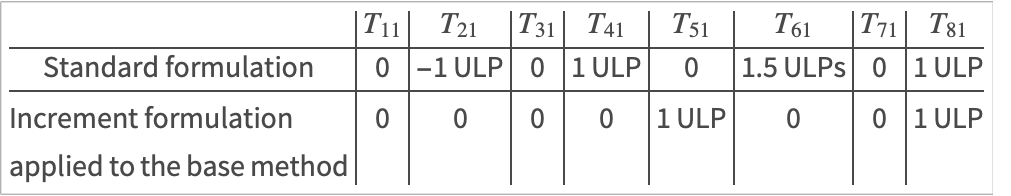
Notice that the rounding-error model that was used to motivate the study of rounding-error growth is limited because in practice, errors in ![]() can exceed 1 ULP.
can exceed 1 ULP.
The increment formulation used throughout the extrapolation process produces rounding errors in ![]() that are smaller than 1 ULP.
that are smaller than 1 ULP.
Method Comparison
This compares the work required for extrapolation based on "ExplicitEuler" (red), the "ExplicitMidpoint" (blue), and "ExplicitModifiedMidpoint" (green).
All computations are carried out using software arithmetic with 32 decimal digits.
Order Selection
system = GetNDSolveProblem["Pleiades"];OrderMonitor[t_, method_NDSolve`Extrapolation] :=
Sow[{t, method["DifferenceOrder"]}];data =
Reap[
NDSolve[system, Method -> {"Extrapolation", Method -> "ExplicitModifiedMidpoint"}, "MethodMonitor" :> OrderMonitor[T, NDSolve`Self]]
][[-1, 1]];ListLinePlot[data]Method Comparison
system = GetNDSolveProblem["Arenstorf"];sol = NDSolve[system, Method -> "StiffnessSwitching", WorkingPrecision -> 32];
refsol = First[FinalSolutions[system, sol]];methods = {{"ExplicitRungeKutta", "StiffnessTest" -> False}, {"Extrapolation", Method -> "ExplicitModifiedMidpoint", "StiffnessTest" -> False}};data = Table[Map[Rest, CompareMethods[system, refsol, methods, AccuracyGoal -> tol, PrecisionGoal -> tol]], {tol, 4, 14}];ListLogLogPlot[Transpose[data], Joined -> True, Axes -> False, Frame -> True, PlotStyle -> {{Green}, {Red}}]Stiff Systems
system = GetNDSolveProblem["VanderPol"];
vars = system["DependentVariables"];
time = system["TimeData"];vdpsol = Flatten[vars /. NDSolve[system, Method -> {"Extrapolation", Method -> "ExplicitModifiedMidpoint"}]]vdpsol = Flatten[vars /. NDSolve[system, Method -> {"Extrapolation", Method -> "LinearlyImplicitEuler"}]]Notice that the Jacobian matrix is computed automatically (user-specifiable by using either numerical differences or symbolic derivatives) and appropriate linear algebra routines are selected and invoked at run time.
Plot[Evaluate[First[vdpsol]], Evaluate[time], Frame -> True, Axes -> False]StepDataPlot[vdpsol]High-Precision Comparison
system = GetNDSolveProblem["Lorenz"];Timing[
erksol = NDSolve[system, Method -> {"ExplicitRungeKutta", "DifferenceOrder" -> 9}, WorkingPrecision -> 32];
]Timing[
adamssol = NDSolve[system, Method -> "Adams", WorkingPrecision -> 32];
]Timing[
extrapsol = NDSolve[system, Method -> {"Extrapolation", Method -> "ExplicitModifiedMidpoint"}, WorkingPrecision -> 32];
]methods = {"ExplicitRungeKutta", "Adams", "Extrapolation"};
solutions = {erksol, adamssol, extrapsol};
MapThread[StepDataPlot[#2, PlotLabel -> #1]&, {methods, solutions}]Mass Matrix - fem2ex
Consider the partial differential equation:
Given an integer ![]() define
define ![]() and approximate at
and approximate at ![]() with
with ![]() using the Galerkin discretization,
using the Galerkin discretization,
where ![]() is a piecewise linear function that is
is a piecewise linear function that is ![]() at
at ![]() and
and ![]() at
at ![]() .
.
The discretization (51) applied to (52) gives rise to a system of ordinary differential equations with constant mass matrix formulation as in (53). The ODE system is the fem2ex problem in [SR97] and is also found in the IMSL library.
n = 9;
h = N[π / (n + 1)];
amat = SparseArray[{Band[{1, 1}] -> 2 h  / 3, Band[{1, 2}] -> h / 6, Band[{2, 1}] -> h / 6}, {n + 2, n + 2}, 0.];
rmat = SparseArray[{Band[{1, 1}] -> -2 / h, Band[{1, 2}] -> 1 / h, Band[{2, 1}] -> 1 / h}, {n + 2, n + 2}, 0.];
vars = {y[t]};
eqs = {amat.y'[t] == rmat.(Exp[t]y[t])};
ics = {y[0] == Table[Sin[k h], {k, 0, n + 1}]};
system = {eqs, ics};
time = {t, 0, π};sollim = NDSolve[system, vars, time, Method -> {"Extrapolation", Method -> "LinearlyImplicitEuler"},
"SolveDelayed" -> "MassMatrix", MaxStepFraction -> 1];StepDataPlot[sollim]soldae = NDSolve[system, vars, time, MaxStepFraction -> 1];StepDataPlot[soldae]PlotSolutionsOn3DGrid[{ndsol_}, opts___ ? OptionQ] :=
Module[{if, m, n, sols, tvals, xvals},
tvals = First[Head[ndsol]["Coordinates"]];
sols = Transpose[ndsol /. t -> tvals];
m = Length[tvals];
n = Length[sols];
xvals = Range[0, n - 1];
data = Table[{{Part[tvals, j], Part[xvals, i]}, Part[sols, i, j]}, {j, m}, {i, n}];
data = Apply[Join, data];
if = Interpolation[data];
Plot3D[Evaluate[if[t, x]], Evaluate[{t, First[tvals], Last[tvals]}], Evaluate[{x, First[xvals], Last[xvals]}], PlotRange -> All, Boxed -> False, opts]
];femsol = PlotSolutionsOn3DGrid[vars /. First[sollim], Ticks -> {Table[i π, {i, 0, 1, 1 / 2}], Range[0, n + 1], Automatic},
AxesLabel -> {"time ", "index", RawBoxes[RotationBox["solution
", BoxRotation -> Pi / 2]]}, Mesh -> {19, 9}, MaxRecursion -> 0, PlotStyle -> None]Fine-Tuning
"StepSizeSafetyFactors"
As with most methods, there is a balance between taking too small a step and trying to take too big a step that will be frequently rejected. The option "StepSizeSafetyFactors"->{s1,s2} constrains the choice of step size as follows. The step size chosen by the method for order ![]() satisfies:
satisfies:
This includes both an order-dependent factor and an order-independent factor.
"StepSizeRatioBounds"
The option "StepSizeRatioBounds"->{srmin,srmax} specifies bounds on the next step size to take such that
"OrderSafetyFactors"
An important aspect in "Extrapolation" is the choice of order.
Each extrapolation step ![]() has an associated work estimate
has an associated work estimate ![]() .
.
The work estimate for explicit base methods is based on the number of function evaluations and the step sequence used.
The work estimate for linearly implicit base methods also includes an estimate of the cost of evaluating the Jacobian, the cost of an LU decomposition, and the cost of backsolving the linear equations.
Estimates for the work per unit step are formed from the work estimate ![]() and the expected new step size to take for a method of order
and the expected new step size to take for a method of order ![]() (computed from (54)):
(computed from (54)): ![]() .
.
Comparing consecutive estimates, ![]() allows a decision about when a different order method will be more efficient.
allows a decision about when a different order method will be more efficient.
The option "OrderSafetyFactors"->{f1,f2} specifies safety factors to be included in the comparison of estimates ![]() .
.
An order decrease is made when ![]() .
.
An order increase is made when ![]() .
.
There are some additional restrictions, such as when the maximal order increase per step is one (two for symmetric methods), and when an increase in order is prevented immediately after a rejected step.
For a nonstiff base method the default values are {4/5,9/10} whereas for a stiff method they are {7/10,9/10}.
Option Summary
option name | default value | |
| "ExtrapolationSequence" | Automatic | specify the sequence to use in extrapolation |
| "MaxDifferenceOrder" | Automatic | specify the maximum order to use |
| Method | "ExplicitModifiedMidpoint" | specify the base integration method to use |
| "MinDifferenceOrder" | Automatic | specify the minimum order to use |
| "OrderSafetyFactors" | Automatic | specify the safety factors to use in the estimates for adaptive order selection |
| "StartingDifferenceOrder" | Automatic | specify the initial order to use |
| "StepSizeRatioBounds" | Automatic | specify the bounds on a relative change in the new step size |
| "StepSizeSafetyFactors" | Automatic | specify the safety factors to incorporate into the error estimate used for adaptive step sizes |
| "StiffnessTest" | Automatic | specify whether to use the stiffness detection capability |
Options of the method "Extrapolation".
The default setting of Automatic for the option "ExtrapolationSequence" selects a sequence based on the stiffness and symmetry of the base method.
The default setting of Automatic for the option "MaxDifferenceOrder" bounds the maximum order by two times the decimal working precision.
The default setting of Automatic for the option "MinDifferenceOrder" selects the minimum number of two extrapolations starting from the order of the base method. This also depends on whether the base method is symmetric.
The default setting of Automatic for the option "OrderSafetyFactors" uses the values {7/10,9/10} for a stiff base method and {4/5,9/10} for a nonstiff base method.
The default setting of Automatic for the option "StartingDifferenceOrder" depends on the setting of "MinDifferenceOrder" ![]() . It is set to
. It is set to ![]() or
or ![]() depending on whether the base method is symmetric.
depending on whether the base method is symmetric.
The default setting of Automatic for the option "StepSizeRatioBounds" uses the values {1/10,4} for a stiff base method and {1/50,4} for a nonstiff base method.
The default setting of Automatic for the option "StepSizeSafetyFactors" uses the values {9/10,4/5} for a stiff base method and {9/10,13/20} for a nonstiff base method.
The default setting of Automatic for the option "StiffnessTest" indicates that the stiffness test is activated if a nonstiff base method is used.
option name | default value | |
| "StabilityTest" | True | specify whether to carry out a stability test on consecutive implicit solutions (see e.g. (55)) |
Options of the method "LinearlyImplicitEuler", "LinearlyImplicitMidpoint", and "LinearlyImplicitModifiedMidpoint".