- See Also
-
Related Guides
- Equation Solving
- Differential Equations
- Partial Differential Equations
- Solvers over Regions
- Geometric Computation
- Mesh-Based Geometric Regions
- Systems Modeling
- Symbolic Vectors, Matrices and Arrays
- Physics & Chemistry: Data and Computation
- Numerical Evaluation & Precision
- Calculus
- Differential Operators
- Scientific Models
- Life Sciences & Medicine: Data & Computation
- Matrix Decompositions
-
Tech Notes
- Numerical Differential Equations
- Numerical Solution of Differential Equations
- Advanced Numerical Differential Equation Solving in the Wolfram Language
- Numerical Mathematics in the Wolfram Language
- PDE Models Overview
- Symbolic Solution of Differential Equations
- Implementation notes: Numerical and Related Functions
-
- See Also
-
Related Guides
- Equation Solving
- Differential Equations
- Partial Differential Equations
- Solvers over Regions
- Geometric Computation
- Mesh-Based Geometric Regions
- Systems Modeling
- Symbolic Vectors, Matrices and Arrays
- Physics & Chemistry: Data and Computation
- Numerical Evaluation & Precision
- Calculus
- Differential Operators
- Scientific Models
- Life Sciences & Medicine: Data & Computation
- Matrix Decompositions
-
Tech Notes
- Numerical Differential Equations
- Numerical Solution of Differential Equations
- Advanced Numerical Differential Equation Solving in the Wolfram Language
- Numerical Mathematics in the Wolfram Language
- PDE Models Overview
- Symbolic Solution of Differential Equations
- Implementation notes: Numerical and Related Functions
NDSolve[eqns,u,{x,xmin,xmax}]
finds a numerical solution to the ordinary differential equations eqns for the function u with the independent variable x in the range xmin to xmax.
NDSolve[eqns,u,{x,xmin,xmax},{y,ymin,ymax}]
solves the partial differential equations eqns over a rectangular region.
NDSolve[eqns,u,{x,y}∈Ω]
solves the partial differential equations eqns over the region Ω.
NDSolve[eqns,u,{t,tmin,tmax},{x,y}∈Ω]
solves the time-dependent partial differential equations eqns over the region Ω.
NDSolve[eqns,{u1,u2,…},…]
solves for the functions ui.


NDSolve
NDSolve[eqns,u,{x,xmin,xmax}]
finds a numerical solution to the ordinary differential equations eqns for the function u with the independent variable x in the range xmin to xmax.
NDSolve[eqns,u,{x,xmin,xmax},{y,ymin,ymax}]
solves the partial differential equations eqns over a rectangular region.
NDSolve[eqns,u,{x,y}∈Ω]
solves the partial differential equations eqns over the region Ω.
NDSolve[eqns,u,{t,tmin,tmax},{x,y}∈Ω]
solves the time-dependent partial differential equations eqns over the region Ω.
NDSolve[eqns,{u1,u2,…},…]
solves for the functions ui.
Details and Options
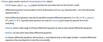
- NDSolve is a numerical differential equation solver that gives results in terms of InterpolatingFunction objects.
- NDSolve[eqns,u[x],{x,xmin,xmax}] gives solutions for u[x] rather than for the function u itself.
- Differential equations must be stated in terms of derivatives such as u'[x], obtained with D, not total derivatives obtained with Dt.
- Partial differential equations may also be specified using the differential operators Grad (∇), Div (∇.), Laplacian (∇2), and Curl (∇). Typically these operators are used as in Inactive[op] to keep the operator form from evaluating.
- NDSolve solves a wide range of ordinary differential equations as well as many partial differential equations.
- NDSolve can also solve many delay differential equations.
- In ordinary differential equations, the functions ui must depend only on the single variable t. In partial differential equations, they may depend on more than one variable.
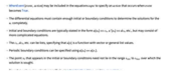
- WhenEvent[event,action] may be included in the equations eqns to specify an action that occurs when event becomes True.
- The differential equations must contain enough initial or boundary conditions to determine the solutions for the ui completely.
- Initial and boundary conditions are typically stated in the form u[x0]==c0, u'[x0]==dc0, etc., but may consist of more complicated equations.
- The c0, dc0, etc. can be lists, specifying that u[x] is a function with vector or general list values.
- Periodic boundary conditions can be specified using u[x0]==u[x1].
- The point x0 that appears in the initial or boundary conditions need not lie in the range xmin to xmax over which the solution is sought.
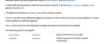
- Boundary values may also be specified using DirichletCondition and NeumannValue.
- In delay differential equations, initial history functions are given in the form u[x/;x<x0]==c0, where c0 is in general a function of x.
- The differential equations in NDSolve can involve complex numbers.
- NDSolve can solve many differential‐algebraic equations, in which some of the eqns are purely algebraic, or some of the variables are implicitly algebraic.
- The ui can be functions of the dependent variables and need not include all such variables.
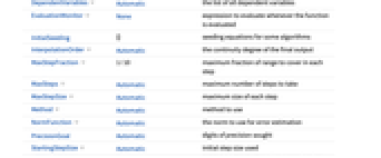
- The following options can be given:
-
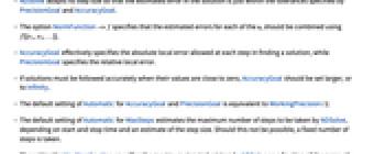
AccuracyGoal Automatic digits of absolute accuracy sought Compiled Automatic whether expressions should be compiled automatically DependentVariables Automatic the list of all dependent variables EvaluationMonitor None expression to evaluate whenever the function is evaluated InitialSeeding {} seeding equations for some algorithms InterpolationOrder Automatic the continuity degree of the final output MaxStepFraction 1/10 maximum fraction of range to cover in each step MaxSteps Automatic maximum number of steps to take MaxStepSize Automatic maximum size of each step Method Automatic method to use NormFunction Automatic the norm to use for error estimation PrecisionGoal Automatic digits of precision sought StartingStepSize Automatic initial step size used StepMonitor None expression to evaluate when a step is taken WorkingPrecision MachinePrecision precision to use in internal computations - NDSolve adapts its step size so that the estimated error in the solution is just within the tolerances specified by PrecisionGoal and AccuracyGoal.
- The option NormFunction->f specifies that the estimated errors for each of the ui should be combined using f[{e1,e2,…}].
- AccuracyGoal effectively specifies the absolute local error allowed at each step in finding a solution, while PrecisionGoal specifies the relative local error.
- If solutions must be followed accurately when their values are close to zero, AccuracyGoal should be set larger, or to Infinity.
- The default setting of Automatic for AccuracyGoal and PrecisionGoal is equivalent to WorkingPrecision/2.
- The default setting of Automatic for MaxSteps estimates the maximum number of steps to be taken by NDSolve, depending on start and stop time and an estimate of the step size. Should this not be possible, a fixed number of steps is taken.
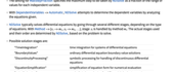
- The setting for MaxStepFraction specifies the maximum step to be taken by NDSolve as a fraction of the range of values for each independent variable.
- With DependentVariables->Automatic, NDSolve attempts to determine the dependent variables by analyzing the equations given.
- NDSolve typically solves differential equations by going through several different stages, depending on the type of equations. With Method->{s1->m1,s2->m2,…}, stage si is handled by method mi. The actual stages used and their order are determined by NDSolve, based on the problem to solve.
- Possible solution stages are:
-
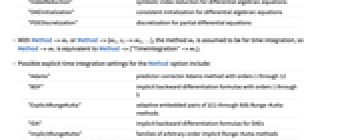
"TimeIntegration" time integration for systems of differential equations "BoundaryValues" ordinary differential equation boundary value solutions "DiscontinuityProcessing" symbolic processing for handling of discontinuous differential equations "EquationSimplification" simplification of equation form for numerical evaluation "IndexReduction" symbolic index reduction for differential algebraic equations "DAEInitialization" consistent initialization for differential algebraic equations "PDEDiscretization" discretization for partial differential equations - With Method->m1 or Method->{m1,s2->m2,…}, the method m1 is assumed to be for time integration, so Method->m1 is equivalent to Method->{"TimeIntegration"->m1}.
- Possible explicit time integration settings for the Method option include:
-
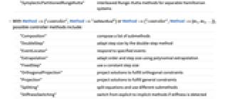
"Adams" predictor‐corrector Adams method with orders 1 through 12 "BDF" implicit backward differentiation formulas with orders 1 through 5 "ExplicitRungeKutta" adaptive embedded pairs of 2(1) through 9(8) Runge–Kutta methods "IDA" implicit backward differentiation formulas for DAEs "ImplicitRungeKutta" families of arbitrary‐order implicit Runge–Kutta methods "SymplecticPartitionedRungeKutta" interleaved Runge–Kutta methods for separable Hamiltonian systems - With Method->{"controller",Method->"submethod"} or Method->{"controller",Method->{m1,m2,…}}, possible controller methods include:
-
"Composition" compose a list of submethods "DoubleStep" adapt step size by the double‐step method "EventLocator" respond to specified events "Extrapolation" adapt order and step size using polynomial extrapolation "FixedStep" use a constant step size "OrthogonalProjection" project solutions to fulfill orthogonal constraints "Projection" project solutions to fulfill general constraints "Splitting" split equations and use different submethods "StiffnessSwitching" switch from explicit to implicit methods if stiffness is detected - Methods used mainly as submethods include:
-
"ExplicitEuler" forward Euler method "ExplicitMidpoint" midpoint rule method "ExplicitModifiedMidpoint" midpoint rule method with Gragg smoothing "LinearlyImplicitEuler" linearly implicit Euler method "LinearlyImplicitMidpoint" linearly implicit midpoint rule method "LinearlyImplicitModifiedMidpoint" linearly implicit Bader‐smoothed midpoint rule method "LocallyExact" numerical approximation to locally exact symbolic solution - The setting InterpolationOrder->All specifies that NDSolve should generate solutions that use interpolation of the same order as the underlying method used. »
Examples
open all close allBasic Examples (7)
Solve a first-order ordinary differential equation:
Use the function and its derivative in a plot:
Second-order nonlinear ordinary differential equation:
Plot the function and its first two derivatives:
System of ordinary differential equations:
Solve the heat equation in one dimension:
Solve the Poisson equation over a Disk:
Find a minimal surface over a Disk with a sinusoidal boundary condition.
Solve a coupled nonlinear sine-Gordon equation over a region.
Scope (28)
Ordinary Differential Equations (8)
Specify any order equation. Reduction to normal form is done automatically:
Directly differentiate the solution to make a phase plot:
Directly specify a system of equations:
Solve for a vector-valued function:
Plot the four components of the solution:
Different equivalent ways of specifying a harmonic oscillator as a second-order equation:
As a system of first-order equations:
Using a vector variable with the dimension deduced from the initial condition:
Use matrix-valued variables to compute the fundamental matrix solution:
Compare to the exact solution:
Define a Van der Pol equation:
The solution's "stiff" behavior that the default solver automatically handles:
Other methods may not be able to solve this system:
Equations can have multiple distinct solutions:
The solution y[x] is continuous, as it integrates the piecewise function once:
The solution y[x] is differentiable, whereas y'[x] is continuous only:
Partial Differential Equations (5)
Nonlinear advection-diffusion equation in one dimension:
Define a system of PDEs of mixed parabolic-hyperbolic type:
Nonlinear sine-Gordon equation in two spatial dimensions with periodic boundary conditions:
Plot the solution at the final time:
Plot the time evolution of a radial cross section of the solution:
Solve a wave equation over a region with a slit:
Solve a Poisson equation with periodic boundary conditions on curved boundaries:
Boundary Value Problems (5)
A nonlinear multipoint boundary value problem:
Solve a nonlinear diffusion equation ![]() with Dirichlet and Neumann boundary conditions starting from an initial seed of
with Dirichlet and Neumann boundary conditions starting from an initial seed of ![]() .
.
Solve a nonlinear equation ![]() with Dirichlet boundary conditions starting from an initial seed of
with Dirichlet boundary conditions starting from an initial seed of ![]() .
.
Solve a complex-valued nonlinear reaction equation ![]() with Dirichlet boundary conditions:
with Dirichlet boundary conditions:
Delay Differential Equations (2)
Hybrid and Discontinuous Equations (4)
Differential-Algebraic Equations (4)
Solve a differential equation with ![]() as an algebraic constraint:
as an algebraic constraint:
Solve an ode system with a singular mass matrix:
The determinant of the Jacobian is zero; the derivative of ![]() is not present:
is not present:
Rewrite the equation as a DAE with an algebraic constraint:
Solve a system of differential equation with singular mass-matrix as a DAE:
Inspect the singularity of the mass matrix:
Solve a DAE by converting it to an index-0 system and solve it as an ODE with invariants:
Options (31)
AccuracyGoal and PrecisionGoal (1)
DependentVariables (1)
EvaluationMonitor (2)
InitialSeedings (2)
InterpolationOrder (1)
Use InterpolationOrder->All to get interpolation the same order as the method:
This is more time-consuming than the default interpolation order used:
MaxStepFraction (1)
Features with small relative size in the integration interval can be missed:
Use MaxStepFraction to ensure features are not missed, independent of interval size:
MaxSteps (1)
MaxStepSize (2)
The default step control may miss a suddenly varying feature:
A smaller MaxStepSize setting ensures that NDSolve catches the feature:
Attempting to compute the number of positive integers less than ![]() misses several events:
misses several events:
Setting a small enough MaxStepSize ensures that none of the events are missed:
Method (14)
TimeIntegration (5)
Specify an explicit Runge–Kutta method to be used for the time integration of a differential equation:
Specify an explicit Runge–Kutta method of order 8 to be used for the time integration:
Specify an explicit Euler method to be used for the time integration of a differential equation:
Show differences between values of x at successive steps with the default solution method:
An explicit Runge–Kutta method changes the step size less often:
PDEDiscretization (3)
Solutions of Burgers' equation may steepen, leading to numerical instability:

Specify a spatial discretization sufficiently fine to resolve the front:
After the front forms, the solution decays relatively rapidly:
Specify use of the finite element method for spatial discretization:
Solve a time-dependent Schrödinger equation on a refined mesh:
BoundaryValues (1)
DiscontinuityProcessing (1)
NDSolve automatically does processing for discontinuous functions like Sign:
If the processing is turned off, NDSolve may fail at the discontinuity point:
With some time integration methods, the solution may be very inaccurate:
An equivalent way to find the solution is to use "DiscontinuitySignature":
The solutions are effectively identical:
The discontinuity signature is 0 when the solution is in sliding mode:
EquationSimplification (2)
The solution cannot be completed because the square root function is not sufficiently smooth:
One solution can be found by forming a residual and solving as a DAE system:
The other solution branch can be given by specifying a consistent value of ![]() :
:
With the suboption "SimplifySystem"->True, NDSolve uses symbolic solutions for components with a sufficiently simple form:
IndexReduction (1)
An index 3 formulation of a constrained pendulum using index reduction:
The default method can only solve index 1 problems:
The problem resulting from symbolic index reduction can be solved:
Solve using reduction to index 0 and a projection method to maintain the constraints:
Plot implicit energy constraint for the two solutions at the time steps:
DAEInitialization (1)
Use forward collocation for initialization to avoid problems with the Abs term at 0:
NormFunction (1)
StartingStepSize (1)
StepMonitor (3)
WorkingPrecision (1)
Error in the solution to a harmonic oscillator over 100 periods:
When the working precision is increased, the local tolerances are correspondingly increased:
With a large working precision, sometimes the "Extrapolation" method is quite effective:
Error in the solution to a harmonic oscillator over 100 periods:
When the working precision is increased, the local tolerances are correspondingly increased:
With a large working precision, sometimes the "Extrapolation" method is quite effective:
Applications (35)
Ordinary Differential Equations (5)
Simulate Duffing's equation for a particle in a double potential well:
The solution depends strongly on initial conditions:
The Lorenz equations [more info]:
The Lotka–Volterra predator-prey equations [more info]:
Look at the appearance of the blue sky catastrophe orbit in the Gavrilov–Shilnikov model:
Reduced 3-body problem [more info]:
A formulation suitable for a number of different initial conditions:
Partial Differential Equations (10)
A large collection of PDE models from various fields with extensive explanation can found in the PDE models overview.
Simple model for soil temperature at depth x with periodic heating at the surface:
Simple wave evolution with periodic boundary conditions:
Wolfram's nonlinear wave equation [more info]:
Wolfram's nonlinear wave equation in two space dimensions:
A soliton profile perturbed by a periodic potential in a nonlinear Schrödinger equation:
Use Stokes's equation to compute the fluid velocity field in a narrowing channel:
Model a temperature field with a heat source in a rod:
Define model variables vars for a transient acoustic pressure field with model parameters pars:
Define initial conditions ics of a right-going sound wave ![]() :
:
Set up the equation with a sound hard boundary at the right end:
Visualize the sound field in the time domain:
Model a 1D chemical species transport through different material with a reaction rate in one. The right side and left side are subjected to a mass concentration and inflow condition, respectively:
Set up the stationary mass transport model variables vars:
Specify the mass transport model parameters species diffusivity ![]() and a reaction rate
and a reaction rate ![]() active in the region
active in the region ![]() :
:
Specify a species flux boundary condition:
Delay Differential Equations (1)
Hybrid Differential Equations (5)
Simulate a bouncing ball that retains 95% of its velocity in each bounce:
Model a ball bouncing down steps:
Each time a linear oscillator solution crosses the negative ![]() axis, reflect it across the
axis, reflect it across the ![]() axis:
axis:
The solution of this reset oscillator exhibits chaotic behavior:
Plot the solution on the negative ![]() axis with a histogram of the reflection points:
axis with a histogram of the reflection points:
Model a one-degree-of-freedom impact oscillator with sinusoidal forcing:
Model a damped oscillator that gets a kick at regular time intervals:
Mechanical Systems (3)
Model the motion of a pendulum in Cartesian coordinates. Derive the governing equations using Newton's second law of motion, ![]() and
and ![]() , with a force diagram:
, with a force diagram:
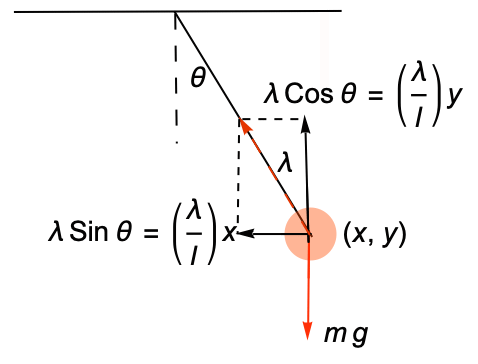
Add damping to the pendulum so that it slows down over time:
The pendulum stabilizes at the vertical fixed point:
Change the rod to a stiff spring by modifying the constraint ![]() :
:
The solution contains high-frequency spring oscillations:
Model a double pendulum of unit mass and length that is released from the horizontal plane. Begin by deriving the equations of motion using Newton's second law:
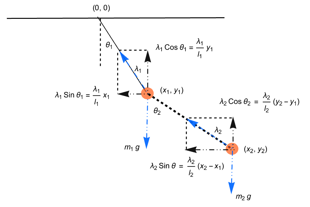
Simulate the system by enforcing the equations and constraints as invariants:
Visualize the motion of the double pendulum:
Model a block on a moving conveyor belt anchored to a wall by a spring using different models for the friction force ![]() , including viscous, Coulomb, Stribeck, and static. Compare positions and velocities for the different models:
, including viscous, Coulomb, Stribeck, and static. Compare positions and velocities for the different models:
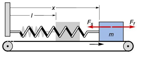
Newton's equation for the block:
Viscous friction is proportional to the relative velocity ![]() :
:
The block stabilizes just above the spring's natural length of 1:
Coulomb friction is proportional to the sign of relative velocity ![]() :
:
The block moves with the belt until the spring force is strong enough:
Stribeck friction is a refined Coulomb friction ![]() :
:
The variation at low velocities is slightly reduced:
Static friction holds the block in place until the spring force exceeds some value μ depending on roughness of surfaces. Use the discrete variable stuck set to 1 when the block is stuck and 0 otherwise:
Check whether the spring force is smaller than μ, and if the block is not moving relative to the belt:
The block repeatedly sticks to the belt, then slips away due to the spring force:
Electrical Systems (6)
Simulate the response of an RLC circuit to a step in the voltage ![]() at time
at time ![]() :
:
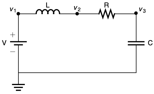
Use component laws together with Kirchhoff's laws for connections:
Simulate the response of an RLC circuit to a step in the voltage ![]() at time
at time ![]() :
:
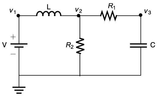
Simulate the behavior of a parallel RLC circuit:
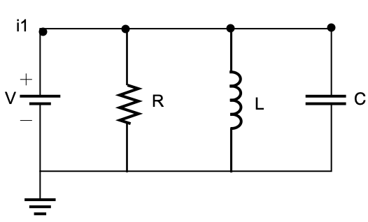
Show the response under a constant input current:
Show the currents in the R, L, C components and the resulting voltage:
Model a transistor-amplifier circuit:
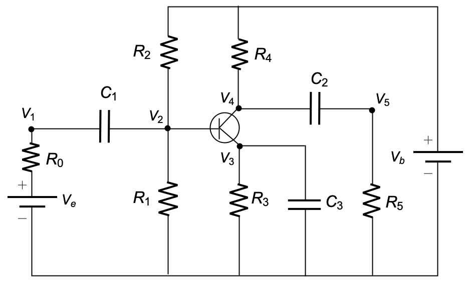
The input voltage ![]() varies sinusoidally:
varies sinusoidally:
The transistor dispatches the voltage in a nonlinear way, depending on ![]() :
:
Use Ohm's law and Kirchhoff's law to determine the governing equations for each node:
Simulate the singular system of equations:
The transistor amplifies voltage ![]() relative to
relative to ![]() :
:
Model a DC-to-DC boost converter from input voltage level vi to desired output voltage level vd using a pulse-width modulated feedback control q[t]:

Use Kirchhoff's laws to get a model for the circuit above:
The control signal q[t] will switch the transistor on for a fraction vi/vd of each period τ:
Boost from a lower voltage vi=24 to a higher voltage vd=36:
Model a DC-to-DC buck-boost converter from input voltage level vi to desired output voltage level vo using a pulse-width modulated feedback control q[t]:

Use Kirchhoff's laws to get a model for the circuit above:
The control signal q[t] will switch the transistor on for a fraction vd/(vi+vd) of each period:
Hydraulic Systems (3)
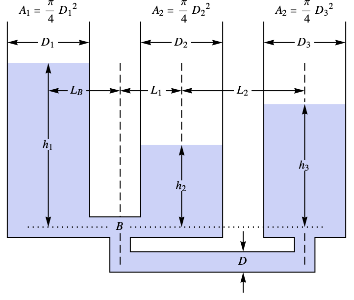
Model the change in height of water in two cylindrical tanks as water flows from one tank to another through a pipe:
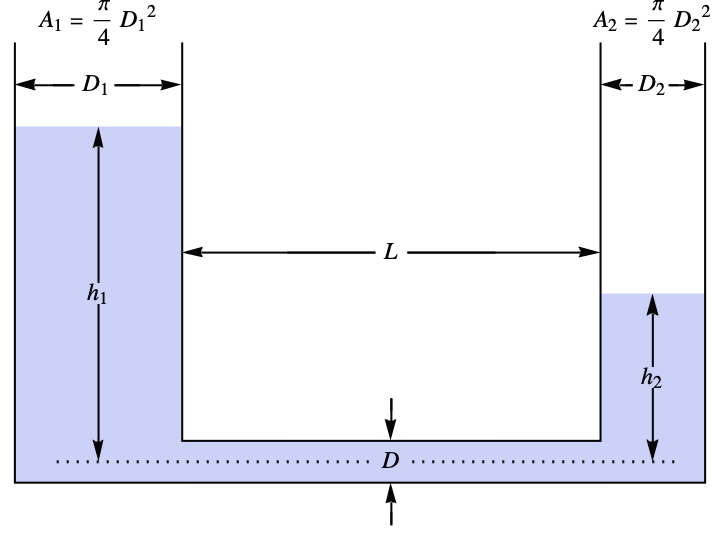
Use pressure relations ![]() and mass conservation:
and mass conservation:
Model the flow across the pipe with the Hagen–Poiseuille relation:
Model the second tank as a leaky tank:
Due to the leak in the second tank, both tanks will eventually drain out:
Model the change in height of water in two hemispherical tanks as water flows from one tank to another through a pipe:
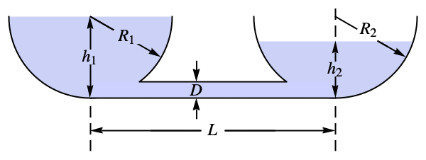
Model the change in height of water in three tanks such that one tank feeds water to the other tanks:
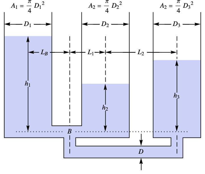
Model the flow across the pipe with the Hagen–Poiseuille relation:
The flow rate from the first pipe will equal the sum of the flow rates in other two pipes:
Model the third tank as a leaky tank:
The first two tanks reach equilibrium and then drain at the same rate:
Chemical Systems (2)
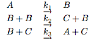
Model the kinetics of an autocatalytic reaction:
The rate equations are given as:
The concentration of the species a, b, c should always be a constant:
Solve and visualize the evolution of the three species:
Model a chemical process of two species, FLB and ZHU, that are continuously mixed with carbon dioxide:
The inflow of carbon dioxide per volume unit is denoted by:
The rate equations are given as:
Equilibrium equation is given as:
Solve the equations and determine the concentration change in FLB, ZHU, CO2, and ZLA:
Properties & Relations (7)
Symbolic versus numerical differential equation solving:
The defining equation for JacobiSN:
Numerically compute values of an integral at different points in an interval:
For functions of the independent variable, NDSolve effectively gives an indefinite integral:
Finding an event is related to finding a root of a function of the solution:
Event location finds the root accurately and efficiently:
This gives ![]() as a function of
as a function of ![]() for a differential equation:
for a differential equation:
Solve the equivalent boundary value problem:
Use NDSolve as a solver for a SystemModel:
Plot variables from the simulation result:
Use SystemModel to model larger hierarchical models:
Possible Issues (14)
Many NDSolve messages have specific message reference pages implemented. See how to access them in the Understand Error Messages workflow.
Numerical Error (4)
The error tends to grow as you go further from the initial conditions:
Find the difference between numerical and exact solutions:
Error for a nonlinear equation:
For high-order methods, the default interpolation may have large errors between steps:
Interpolation with the order corresponding to the method reduces the error between steps:
Some of the algorithms the finite element method uses are not deterministic. This means some randomness is used during these algorithms and will result in slightly different results if the same input is run:
Solve the same PDE twice. There can be a small difference in the solutions:
Differential Algebraic Equations (3)
NDSolve cannot automatically handle systems of index greater than 1:
High-index systems can be solved by performing index reduction on the system:
Here is a system of differential-algebraic equations:
NDSolve may change the specified initial conditions if it cannot find the solution with ![]() :
:
Change the initial starting guess for the iterations to avoid such issues:
NDSolve is limited to index 1, but the solution with ![]() has index 2:
has index 2:
To solve high-index systems, use index reduction to reduce the DAE to index 1:
The default method may not be able to converge to the default tolerances:
With lower AccuracyGoal and PrecisionGoal settings, a solution is found:
The "StateSpace" time integration method can solve this with default tolerances:
Partial Differential Equations (4)
A large collection of PDE models from various fields with extensive explanation can found in the PDE models overview.
The spatial discretization is based on the initial value, which varies less than the final value:

By increasing the minimal number of spatial grid points, you can accurately compute the final value:
The plot demonstrates the onset of a spatially more complex solution:
Define a heat equation with an initial value that is a step function:
Discontinuities in the initial value may result in too many spatial grid points:
Setting the number of spatial grid points smaller results in essentially as good a solution:
Define a Laplace equation with initial values:
The solver only works for equations well posed as initial value (Cauchy) problems:

Boundary Value Problems (1)
Tech Notes
-
▪
- Numerical Differential Equations ▪
- Numerical Solution of Differential Equations ▪
- Advanced Numerical Differential Equation Solving in the Wolfram Language ▪
- Numerical Mathematics in the Wolfram Language ▪
- PDE Models Overview ▪
- Symbolic Solution of Differential Equations ▪
- Implementation notes: Numerical and Related Functions
Related Guides
-
▪
- Equation Solving ▪
- Differential Equations ▪
- Partial Differential Equations ▪
- Solvers over Regions ▪
- Geometric Computation ▪
- Mesh-Based Geometric Regions ▪
- Systems Modeling ▪
- Symbolic Vectors, Matrices and Arrays ▪
- Physics & Chemistry: Data and Computation ▪
- Numerical Evaluation & Precision ▪
- Calculus ▪
- Differential Operators ▪
- Scientific Models ▪
- Life Sciences & Medicine: Data & Computation ▪
- Matrix Decompositions
Related Links
History
Introduced in 1991 (2.0) | Updated in 1996 (3.0) ▪ 2003 (5.0) ▪ 2007 (6.0) ▪ 2008 (7.0) ▪ 2012 (9.0) ▪ 2014 (10.0) ▪ 2019 (12.0)
Text
Wolfram Research (1991), NDSolve, Wolfram Language function, https://reference.wolfram.com/language/ref/NDSolve.html (updated 2019).
CMS
Wolfram Language. 1991. "NDSolve." Wolfram Language & System Documentation Center. Wolfram Research. Last Modified 2019. https://reference.wolfram.com/language/ref/NDSolve.html.
APA
Wolfram Language. (1991). NDSolve. Wolfram Language & System Documentation Center. Retrieved from https://reference.wolfram.com/language/ref/NDSolve.html
BibTeX
@misc{reference.wolfram_2025_ndsolve, author="Wolfram Research", title="{NDSolve}", year="2019", howpublished="\url{https://reference.wolfram.com/language/ref/NDSolve.html}", note=[Accessed: 12-May-2026]}
BibLaTeX
@online{reference.wolfram_2025_ndsolve, organization={Wolfram Research}, title={NDSolve}, year={2019}, url={https://reference.wolfram.com/language/ref/NDSolve.html}, note=[Accessed: 12-May-2026]}
