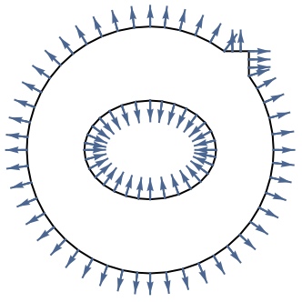
BoundaryUnitNormal[x,y,…]
represents an outward-pointing unit normal vector ![]() on a region.
on a region.


BoundaryUnitNormal
BoundaryUnitNormal[x,y,…]
represents an outward-pointing unit normal vector ![]() on a region.
on a region.
Details and Options
- BoundaryUnitNormal can be used to construct partial differential equation boundary conditions that depend on the unit normal vector
 of the boundary.
 - BoundaryUnitNormal can be used with NeumannValue, DirichletCondition and NIntegrate.
- BoundaryUnitNormal can be generated by boundary conditions like AcousticAbsorbingValue, HeatFluxValue or MassOutflowValue.
- BoundaryUnitNormal can be used to specify a tangential on the boundary.
- BoundaryUnitNormal will evaluate to a vector of length of the embedding dimension of the region
 when the boundary condition is discretized.
 - Components of the boundary unit normal
 can be accessed with Indexed.
 - For finite element approximations, the PDE is multiplied with a test function
 and integrated over
  . Integration by parts gives
  . The integrand
  in the boundary integral is replaced with the NeumannValue
  .
. - When a PDE specifies the Neumann value as
 , BoundaryUnitNormal can be used to model
  instead by specifying the NeumannValue as
  .
. - Conversely, when a PDE specifies the Neumann value as
 , BoundaryUnitNormal can be used to model
  instead by specifying the NeumannValue as
  .
. - At internal boundaries of a region, the boundary unit normal is not uniquely defined.
- The value of the boundary unit normal
 will be computed by solving
  with a Dirichlet condition of
  on all boundaries including internal boundaries over the entire region
  . The boundary unit normal is then the gradient of
  normalized with
  .
.
Examples
open all close allBasic Examples (1)
<<NDSolve`FEM`Solve a Poisson equation on a unit Disk:
solution = NDSolveValue[{-Laplacian[u[x, y], {x, y}] == 1, DirichletCondition[u[x, y] == 0, True]}, u, {x, y}∈Disk[]]Plot3D[solution[x, y], {x, y}∈Disk[]]Compute the total flux through the boundary of the region through a second-order approximation of the boundary region:
NIntegrate[BoundaryUnitNormal[x, y].Grad[-solution[x, y], {x, y}], {x, y}∈ToBoundaryMesh[solution["ElementMesh"], "MeshOrder" -> 2]]Compute the total flux through the boundary of a subregion:
NIntegrate[BoundaryUnitNormal[x, y].Grad[-solution[x, y], {x, y}], {x, y}∈RegionBoundary[Rectangle[{-1 / 2, -1 / 2}, {1 / 2, 1 / 2}]]]Scope (6)
Solve a Poisson equation on a unit Disk:
solution = NDSolveValue[{-Laplacian[u[x, y], {x, y}] == 1, DirichletCondition[u[x, y] == 0, True]}, u, {x, y}∈Disk[]]Compute the total flux through the outer boundary:
-NIntegrate[Grad[solution[x, y], {x, y}].BoundaryUnitNormal[x, y], {x, y}∈RegionBoundary[Disk[]]]Compute the total flux through the boundary of the region through a second-order approximation of the boundary region:
-NIntegrate[Grad[solution[x, y], {x, y}].BoundaryUnitNormal[x, y], {x, y}∈ToBoundaryMesh[solution["ElementMesh"], "MeshOrder" -> 2]]Specify a differential equation and a region:
op = Inactive[Div][-0.075*Inactive[Grad][c[x], {x}], {x}] + 1;
Ω = Line[{{0}, {1}}];
On the left, set up a NeumannValue with a boundary unit normal and solve the equation:
solution1 = NDSolveValue[{
op == NeumannValue[BoundaryUnitNormal[x].{-c[x]}, x == 0]}, c, x∈Ω]Plot[solution1[x], {x}∈Ω]For this domain, the equivalent of the BoundaryUnitNormal at the left is ![]() :
:
solution2 = NDSolveValue[{
	op == NeumannValue[{-1}.{-c[x]}, x == 0]}, c, x∈Ω]
Show that the solutions are equal:
Plot[solution1[x] - solution2[x], {x}∈Ω]Create a tangential for a NeumannValue:
Ω = RegionDifference[Rectangle[{0, 0}, {4, 4}], Disk[]];
solution = NDSolveValue[{Laplacian[u[x, y], {x, y}] == NeumannValue[Cross[BoundaryUnitNormal[x, y]].{1, 1}, x ^ 2 + y ^ 2 == 1], DirichletCondition[u[x, y] == 0, x == 4 && y == 0]}, u, {x, y}∈Ω];
StreamPlot[Evaluate[Grad[solution[x, y], {x, y}]], {x, y}∈Ω]
Make use of a Indexed component of a BoundaryUnitNormal to compute a NeumannValue:
Ω = RegionDifference[Rectangle[{0, 0}, {4, 4}], Disk[]];
solution = NDSolveValue[{Laplacian[u[x, y], {x, y}] == NeumannValue[{-Indexed[BoundaryUnitNormal[x, y], 2], 0}.{1, 1}, x ^ 2 + y ^ 2 == 1], DirichletCondition[u[x, y] == 0, x == 4 && y == 0]}, u, {x, y}∈Ω];
StreamPlot[Evaluate[Grad[solution[x, y], {x, y}]], {x, y}∈Ω]
Solve a Poisson equation on a geometry:
Ω = RegionDifference[RegionUnion[Disk[{0, 0}, 5], Rectangle[{0, 0}, {7, 5}]], Ellipsoid[{0, 0}, {3, 2}]];
solution = NDSolveValue[{-Laplacian[u[x, y], {x, y}] == 1, DirichletCondition[u[x, y] == 0, True]}, u, {x, y}∈Ω]Plot3D[solution[x, y], {x, y}∈Ω]Compute the total flux through the boundary:
NIntegrate[BoundaryUnitNormal[x, y].Grad[-solution[x, y], {x, y}], {x, y}∈ToBoundaryMesh[solution["ElementMesh"], "MeshOrder" -> 2]]Set up a NeumannValue with a boundary normal:
op = D[c[t, x], t] + Inactive[Div][-0.075*Inactive[Grad][c[t, x], {x}], {x}];
ifunNormal = NDSolveValue[{op == NeumannValue[-BoundaryUnitNormal[x].({-1} * c[t, x]), x == 0], c[0, x] == Exp[-100 * (x - 1 / 2) ^ 2]}, c, {t, 0, 2}, x∈Line[{{0}, {1}}]]
Use a Neumann 0 boundary condition and solve the equation again:
ifunNeumannZero = NDSolveValue[{op == NeumannValue[0, x == 0], c[0, x] == Exp[-100 * (x - 1 / 2) ^ 2]}, c, {t, 0, 2}, x∈Line[{{0}, {1}}]]Inspect how the solutions start to differ over time:
Manipulate[Plot[{ifunNormal[t, x], ifunNeumannZero[t, x]}, {x, 0, 1}, PlotRange -> {0, 1}], {t, 0, 2}, SaveDefinitions -> True]For this domain, the equivalent of the BoundaryUnitNormal at the left is ![]() :
:
ifunNormal2 = NDSolveValue[{op == NeumannValue[-{-1}.({-1} * c[t, x]), x == 0], c[0, x] == Exp[-100 * (x - 1 / 2) ^ 2]}, c, {t, 0, 2}, x∈Line[{{0}, {1}}]]Check that the solutions are the same:
Plot3D[ifunNormal[t, x] - ifunNormal2[t, x], {x, 0, 1}, {t, 0, 2}]Applications (1)
The following example considers a Stokes flow with prescribed traction boundary conditions in an annulus region. On the outer edge, at ![]() , there are no-slip boundary conditions. These set the fluid velocity in the
, there are no-slip boundary conditions. These set the fluid velocity in the ![]() and
and ![]() directions to 0,
directions to 0, ![]() . On the inner boundary, at
. On the inner boundary, at ![]() , a traction is prescribed. The traction with the stress vector
, a traction is prescribed. The traction with the stress vector ![]() is given as:
is given as:
Here, ![]() is the radial unit vector given as
is the radial unit vector given as ![]() and
and ![]() is the tangent unit vector given as
is the tangent unit vector given as ![]() .
. ![]() and
and ![]() are the Cartesian unit vectors in the
are the Cartesian unit vectors in the ![]() and
and ![]() directions, respectively. For this example, the traction is set in normal direction to
directions, respectively. For this example, the traction is set in normal direction to ![]() and the tangential traction is set to
and the tangential traction is set to ![]() . In other words, at the inner boundary the velocity is not specified, only the traction
. In other words, at the inner boundary the velocity is not specified, only the traction ![]() is specified.
is specified.
The fluid stress tensor ![]() is given by:
is given by:
Set up parameters, geometry and refined mesh:
pars = <|a -> 1 / 5, b -> 1, μ -> 1|>;
Ω = Annulus[{0, 0}, {a, b}] /. pars;
mesh = ToElementMesh[Ω, "RegionHoles" -> {0, 0}, MeshRefinementFunction -> Function[{vertices, area}, area > 0.000025 (0.1 + 20 Norm[Mean[vertices]])]];
Set up a Stokes flow operator:
op = {Inactive[Div][{{-2 * μ, 0}, {0, -μ}}.Inactive[Grad][u[x, y], {x, y}], {x, y}] +
	Inactive[Div][{{0, 0}, {-μ, 0}}.Inactive[Grad][v[x, y], {x, y}], {x, y}] + Inactive[Div][{1, 0} * p[x, y], {x, y}],
	Inactive[Div][{{0, -μ}, {0, 0}}.Inactive[Grad][u[x, y], {x, y}], {x, y}] +
	Inactive[Div][{{-μ, 0}, {0, -2 * μ}}.Inactive[Grad][v[x, y], {x, y}], {x, y}] +
	Inactive[Div][{0, 1} * p[x, y], {x, y}],
	Derivative[1, 0][u][x, y] + Derivative[0, 1][v][x, y]
	} /. pars;
Set up a no-slip condition on the outer boundary:
ΓWall = DirichletCondition[{u[x, y] == 0, v[x, y] == 0}, ElementMarker == 2]On the inner surface, you can compute the tangent unit normal from the outward-pointing unit normal ![]() with a cross product. Use a cross product to compute the unit tangent from the unit normal vector
with a cross product. Use a cross product to compute the unit tangent from the unit normal vector ![]() :
:
Cross[{Subscript[n, x], Subscript[n, y]}]To extract the first and second components of the cross product for the ![]() and
and ![]() directions, respectively, Indexed is used.
directions, respectively, Indexed is used.
Set up the traction boundary conditions:
Γu = NeumannValue[Indexed[Cross[BoundaryUnitNormal[x, y]], 1] * ((x / a) ^ 2 - (y / a) ^ 2), ElementMarker == 1];
Γv = NeumannValue[Indexed[Cross[BoundaryUnitNormal[x, y]], 2] * ((x / a) ^ 2 - (y / a) ^ 2), ElementMarker == 1];
Equivalently, note that the tangent unit normal can also be given as ![]() because the unit normal vector on the inner surface is
because the unit normal vector on the inner surface is ![]() and the unit tangent then is
and the unit tangent then is ![]() :
:
NeumannValue[(y / a) * ((x / a) ^ 2 - (y / a) ^ 2), ElementMarker == 1];
NeumannValue[-(x / a) * ((x / a) ^ 2 - (y / a) ^ 2), ElementMarker == 1];
Without specifying a boundary condition for the pressure, the pressure value will be floating and NDSolve will give a warning that not enough boundary conditions are specified:
{ufun, vfun, pfun} = NDSolveValue[{op == {Γu, Γv, 0} /. pars, ΓWall}, {u, v, p}, {x, y}∈mesh, Method -> {"FiniteElement", "InterpolationOrder" -> {u -> 2, v -> 2, p -> 1}}, DependentVariables -> {u, v, p}]Visualize the pressure solution and the velocity field:
Show[{DensityPlot[pfun[x, y], {x, y}∈mesh, ...], StreamPlot[{ufun[x, y], vfun[x, y]}, {x, y}∈mesh, ...]}, ...]To verify that the traction boundary condition works, you can compute radial and tangential components of the velocities and plot them at ![]() for all
for all ![]() . For the radial velocity, a solution proportional to
. For the radial velocity, a solution proportional to ![]() is expected, and for the tangential velocity, a solution proportional to
is expected, and for the tangential velocity, a solution proportional to ![]() is expected.
is expected.
Define a function to compute the radial and tangential components of the velocities:
vr[x_, y_] := x / Sqrt[x ^ 2 + y ^ 2] * ufun[x, y] + y / Sqrt[x ^ 2 + y ^ 2] * vfun[x, y]
vt[x_, y_] := -(y / Sqrt[x ^ 2 + y ^ 2]) * ufun[x, y] + x / Sqrt[x ^ 2 + y ^ 2] * vfun[x, y]
Plot the radial component of the velocities and a function proportional to ![]() :
:
Plot[Evaluate[{vr[a * Cos[θ], a * Sin[θ]], -Sin[2θ] * a / 20} /. pars], {θ, 0, 2π}, PlotLegends -> {"vr", "∝ sin(2θ)"}]Plot the tangential component of the velocities and a function proportional to ![]() :
:
Plot[Evaluate[{vt[a * Cos[θ], a * Sin[θ]], -Cos[2θ] * a / 5} /. pars], {θ, 0, 2π}, PlotLegends -> {"vt", "∝ cos(2θ)"}]Next, compute the normal stress and the shear at the inner boundary and check that they match the prescribed traction boundary conditions. The stress tensor is given by:
The normal and tangential components of the traction vector can be computed by
Create a function to compute the stress tensor ![]() :
:
gradU = Grad[{ufun[x, y], vfun[x, y]}, {x, y}];
sigma[x_, y_] := Evaluate[(μ * (gradU + Transpose[gradU]) - pfun[x, y] * IdentityMatrix[2]) /. pars];
Compute the unit normal vector:
normal = ElementMeshBoundaryUnitNormal[mesh]Define a function for the tangent vector:
tangent[x_, y_] := Cross[normal[x, y]]Define a function to compute the normal stress:
normalStress[x_ ? NumberQ, y_ ? NumberQ] := normal[x, y].(sigma[x, y].normal[x, y]);Define a function to compute the shear stress:
shearStress[x_ ? NumberQ, y_ ? NumberQ] := tangent[x, y].(sigma[x, y].normal[x, y]);Visualize the computed normal and shear stress at ![]() :
:
stresses = {normalStress[a * Cos[θ], a * Sin[θ]], shearStress[a * Cos[θ], a * Sin[θ]]} /. pars;
Plot[stresses, {θ, 0, 2 Pi}, ...]
Visualize the difference of the normal and shear stress at ![]() from the boundary conditions:
from the boundary conditions:
Plot[Evaluate[stresses - {0, Cos[2θ]}], {θ, 0, 2 Pi}, ...]Properties & Relations (2)
Compute the boundary unit normal field:
boundaryUnitNormal = ElementMeshBoundaryUnitNormal[ToElementMesh[Disk[]]]Visualize the boundary unit normal:
VectorPlot[boundaryUnitNormal[x, y], {x, y}∈Disk[]]Visualize the boundary unit normal on the boundary only:
VectorPlot[boundaryUnitNormal[x, y], {x, y}∈Disk[], VectorPoints -> ToBoundaryMesh[Disk[]]["Coordinates"]]The boundary unit normal is computed by solving a Poisson equation over the region and specifying 0 Dirichlet conditions. Compute a Poisson equation over a unit Disk:
potential = NDSolveValue[{Laplacian[u[x, y], {x, y}] == 1, DirichletCondition[u[x, y] == 0, True]}, u[x, y], {x, y}∈Disk[], "ExtrapolationHandler" -> {Automatic, "WarningMessage" -> False}];Compute the normalized gradient of the potential:
unitNormal = Normalize[Grad[potential, {x, y}], Sqrt[Total[# ^ 2]]&];VectorPlot[unitNormal, {x, y}∈Disk[]]This is the same as computing the boundary unit normal of an ElementMesh:
boundaryUnitNormal = ElementMeshBoundaryUnitNormal[ToElementMesh[Disk[]]];
VectorPlot[boundaryUnitNormal[x, y], {x, y}∈Disk[]]Text
Wolfram Research (2023), BoundaryUnitNormal, Wolfram Language function, https://reference.wolfram.com/language/FEMDocumentation/ref/BoundaryUnitNormal.html.
CMS
Wolfram Language. 2023. "BoundaryUnitNormal." Wolfram Language & System Documentation Center. Wolfram Research. https://reference.wolfram.com/language/FEMDocumentation/ref/BoundaryUnitNormal.html.
APA
Wolfram Language. (2023). BoundaryUnitNormal. Wolfram Language & System Documentation Center. Retrieved from https://reference.wolfram.com/language/FEMDocumentation/ref/BoundaryUnitNormal.html