


MassFluxValue
MassFluxValue[pred,vars,pars]
represents a mass flux boundary condition for PDEs with predicate pred indicating where it applies, with model variables vars and global parameters pars.
MassFluxValue[pred,vars,pars,lkey]
represents a mass flux boundary condition with local parameters specified in pars[lkey].
Details
- MassFluxValue specifies a boundary condition for MassTransportPDEComponent and is used as part of the modeling equation:
- MassFluxValue is typically used to model mass species flow through a boundary caused by a species source or sink outside of the domain.
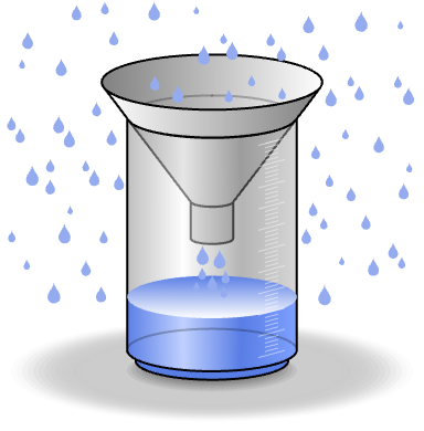
- A flow rate is the flow of a quantity like energy or mass per time. Flux is the flow rate through the boundary and is measured in the units of the quantity per area per time. A millimeter of rain per cross section of opening area per hour is a rain flux.
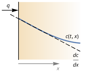
- MassFluxValue models the rate of mass species flowing through some part of the boundary with dependent variable
 in [
in [![TemplateBox[{InterpretationBox[, 1], {"mol", , "/", , {"m", ^, 3}}, moles per meter cubed, {{(, "Moles", )}, /, {(, {"Meters", ^, 3}, )}}}, QuantityTF]](Files/MassFluxValue.en/4.png "TemplateBox[{InterpretationBox[, 1], {\"mol\", , \"/\", , {\"m\", ^, 3}}, moles per meter cubed, {{(, \"Moles\", )}, /, {(, {\"Meters\", ^, 3}, )}}}, QuantityTF]") ], independent variables
], independent variables  in [
in [![TemplateBox[{InterpretationBox[, 1], "m", meters, "Meters"}, QuantityTF]](Files/MassFluxValue.en/6.png "TemplateBox[{InterpretationBox[, 1], \"m\", meters, \"Meters\"}, QuantityTF]") ] and time variable
] and time variable  in [
in [![TemplateBox[{InterpretationBox[, 1], "s", seconds, "Seconds"}, QuantityTF]](Files/MassFluxValue.en/8.png "TemplateBox[{InterpretationBox[, 1], \"s\", seconds, \"Seconds\"}, QuantityTF]") ].
]. - Stationary variables vars are vars={c[x1,…,xn],{x1,…,xn}}.
- Time-dependent variables vars are vars={c[t,x1,…,xn],t,{x1,…,xn}}.
- The non-conservative time-dependent mass transport model MassTransportPDEComponent is based on a convection-diffusion model with mass diffusivity
 , mass convection velocity vector
  , mass reaction rate
  and mass source term
  :
: - The conservative time-dependent mass transport model MassTransportPDEComponent is based on a conservative convection-diffusion model given by:
- In the non-conservative form, MassFluxValue with mass flux
 in
in  and boundary unit normal
  models:
 - In the conservative form, MassFluxValue models:
- Model parameters pars as specified for MassTransportPDEComponent.
- The following additional model parameters pars can be given:
-
parameter default symbol "BoundaryUnitNormal" Automatic 
"MassFlux" 0  , mass flux [
![TemplateBox[{InterpretationBox[, 1], {"mol", , "/(", , "m", , "s", , ")"}, moles per meter second, {{(, "Moles", )}, /, {(, {"Meters", , "Seconds"}, )}}}, QuantityTF]](Files/MassFluxValue.en/23.png "TemplateBox[{InterpretationBox[, 1], {\"mol\", , \"/(\", , \"m\", , \"s\", , \")\"}, moles per meter second, {{(, \"Moles\", )}, /, {(, {\"Meters\", , \"Seconds\"}, )}}}, QuantityTF]") ]
]"ModelForm" "NonConservative" - - All model parameters may depend on any of
 ,
,  and
and  , as well as other dependent variables.
 - To localize model parameters, a key lkey can be specified, and values from association pars[lkey] are used for model parameters.
- MassFluxValue evaluates to a NeumannValue.
- The boundary predicate pred can be specified as in NeumannValue.
- If the MassFluxValue depends on parameters
 that are specified in the association pars as …,keypi…,pivi,…, the parameters
  are replaced with
  .
.
Examples
open all close allBasic Examples (2)
Set up a mass flux boundary condition in non-conservative form:
MassFluxValue[x ≥ 0, {c[t, x], t, {x}}, <|"MassConvectionVelocity" -> {v}, "MassFlux" -> q[t, x]|>]Set up a mass flux boundary condition in conservative form:
MassFluxValue[x ≥ 0, {c[t, x], t, {x}}, <|"ModelForm" -> "Conservative", "MassFlux" -> q[t, x]|>]Scope (10)
Basic Uses (2)
Define model variables vars for a transient species field with model parameters pars and a specific boundary condition parameter:
vars = {c[t, x, y], t, {x, y}};
pars = <|"DiffusionCoefficient" -> 0.026, "MassConvectionVelocity" -> {0.1}, "BoundaryCondition1" -> <|"MassFlux" -> q1|>|>;
MassFluxValue[x == 1, vars, pars, "BoundaryCondition1"]
Define model variables vars for a transient species field with model parameters pars and multiple specific parameter boundary conditions:
vars = {c[t, x, y], t, {x, y}};
pars = <|"DiffusionCoefficient" -> 0.026, "MassConvectionVelocity" -> {0.1}, "BoundaryCondition1" -> <|"MassFlux" -> q1|>, "BoundaryCondition2" -> <|"MassFlux" -> q2|>|>;MassFluxValue[x == 0, vars, pars, "BoundaryCondition1"]MassFluxValue[x == 1, vars, pars, "BoundaryCondition2"]1D (1)
Model a 1D chemical species field in an incompressible fluid whose right side and left side are subjected to a mass concentration and inflow condition, respectively:
Set up the stationary mass transport model variables ![]() :
:
vars = {c[x], {x}};Ω = Line[{{0}, {1}}];Specify the mass transport model parameters species diffusivity ![]() and fluid flow velocity
and fluid flow velocity ![]() :
:
pars = <|"DiffusionCoefficient" -> 0.026, "MassConvectionVelocity" -> {0.1}|>;Specify a species flux boundary condition:
Subscript[Γ, flux] = MassFluxValue[x == 0, vars, pars, <|"MassFlux" -> 1|>]Specify a mass concentration boundary condition:
Subscript[Γ, C] = MassConcentrationCondition[x == 1, vars, pars, <|"MassConcentration" -> 0|>]eqn = MassTransportPDEComponent[vars, pars] == Subscript[Γ, flux]cfun = NDSolveValue[{eqn, Subscript[Γ, C]}, c, x∈Ω];Plot[cfun[x], x∈Ω, Rule[...]]2D (1)
Model mass transport of a pollutant in a 2D rectangular region in an isotropic homogeneous medium. Initially, the pollutant concentration is zero throughout the region of interest. A concentration of 3000 ![]() is maintained at a strip with dimension 0.2
is maintained at a strip with dimension 0.2 ![]() located at the center of the left boundary, while the right boundary is subject to a parallel species flow with a constant concentration of 1500
located at the center of the left boundary, while the right boundary is subject to a parallel species flow with a constant concentration of 1500 ![]() , allowing for mass transfer. A pollutant outflow of 100
, allowing for mass transfer. A pollutant outflow of 100 ![]() is applied at both the top and bottom boundaries. A diffusion coefficient of 0.833
is applied at both the top and bottom boundaries. A diffusion coefficient of 0.833 ![]() is distributed uniformly with a uniform horizontal velocity of 0.01
is distributed uniformly with a uniform horizontal velocity of 0.01 ![]() :
:
Set up the mass transport model variables ![]() :
:
vars = {c[x, y], {x, y}};Set up a rectangular domain with a width of ![]() and a height of
and a height of ![]() :
:
Ω = Rectangle[{0, 0}, {20, 10}];Specify model parameters species diffusivity ![]() and fluid flow velocity
and fluid flow velocity ![]() :
:
pars = <|"DiffusionCoefficient" -> 0.833, "MassConvectionVelocity" -> {0.01, 0}|>;Set up a species concentration source of 0.2 ![]() length at the center of the left surface:
length at the center of the left surface:
Subscript[Γ, concentration] = MassConcentrationCondition[x == 0 && y ≤ 5.1 && y ≥ 4.9, vars, pars, <|"MassConcentration" -> 3000|>]Set up a mass transfer boundary on the right surface:
Subscript[Γ, transfer] = MassTransferValue[x == 20, vars, pars, <|"AmbientConcentration" -> 1500, "MassTransferCoefficient" -> 5|>]Set up an outflow flux ![]() of
of ![]() on the top and bottom surfaces:
on the top and bottom surfaces:
Subscript[Γ, flux] = MassFluxValue[y == 0 || y == 10, vars, pars, <|"MassFlux" -> -100|>]eqn = MassTransportPDEComponent[vars, pars] == Subscript[Γ, transfer] + Subscript[Γ, flux]cfun = NDSolveValue[{eqn, Subscript[Γ, concentration]}, c, {x, y}∈Ω];ContourPlot[cfun[x, y], {x, y}∈Ω, ...]3D (1)
Model a non-conservative chemical species field in a unit cubic domain, with two mass conditions at two lateral surfaces and a mass inflow through a circle with radius 0.2 ![]() at the center of the top surface, as well as an orthotropic mass diffusivity
at the center of the top surface, as well as an orthotropic mass diffusivity ![]() :
:
Set up the mass transport model variables ![]() :
:
vars = {c[x, y, z], {x, y, z}};Ω = Cuboid[{0, 0, 0}, {1, 1, 1}];Specify a diffusivity ![]() and a flow velocity field
and a flow velocity field ![]() :
:
pars = <|"DiffusionCoefficient" -> {{1, 0, 0}, {0, 5, 0}, {0, 0, 10}}, "MassConvectionVelocity" -> {0, 10, 0}|>;Subscript[Γ, CC] = {MassConcentrationCondition[x == 0, vars, <|"MassConcentration" -> 0|>], MassConcentrationCondition[x == 1, vars, <|"MassConcentration" -> 1|>]}Specify a flux condition ![]() of
of ![]() through a regional circle on the top surface:
through a regional circle on the top surface:
Subscript[Γ, flux] = MassFluxValue[z == 1 && (x - 0.5) ^ 2 + (y - 0.5) ^ 2 ≤ 0.04, vars, pars, <|"MassFlux" -> 100|>]eqn = MassTransportPDEComponent[vars, pars] == Subscript[Γ, flux]cfun = NDSolveValue[{eqn, Subscript[Γ, CC]}, c, {x, y, z}∈Ω];GraphicsRow[Table[SliceContourPlot3D[cfun[x, y, z], sl, {x, y, z}∈Ω, ...], {...}]]Material Regions (1)
Model a 1D chemical species transport through different material with a reaction rate in one. The right side and left side are subjected to a mass concentration and inflow condition, respectively:
Set up the stationary mass transport model variables ![]() :
:
vars = {c[x], {x}};Ω = Line[{{0}, {1}}];Specify the mass transport model parameters species diffusivity ![]() and a reaction rate
and a reaction rate ![]() active in the region
active in the region ![]() :
:
pars = <|"DiffusionCoefficient" -> 0.01, "MassReactionRate" -> If[x > 1 / 2, 1, 0]|>;Specify a species flux boundary condition:
Subscript[Γ, flux] = MassFluxValue[x == 0, vars, pars, <|"MassFlux" -> 1|>]Specify a mass concentration boundary condition:
Subscript[Γ, C] = MassConcentrationCondition[x == 1, vars, pars, <|"MassConcentration" -> 0|>]eqn = MassTransportPDEComponent[vars, pars] == Subscript[Γ, flux]cfun = NDSolveValue[{eqn, Subscript[Γ, C]}, c, x∈Ω];Show[Plot[cfun[x], x∈Ω, Rule[...]], Graphics[...]]Time Dependent (1)
Model a 1D non-conservative chemical species field and a mass flux through part of the boundary with:
Set up the time-dependent mass transport model variables ![]() :
:
vars = {c[t, x], t, {x}};Ω = Line[{{0}, {1}}];Specify the mass transport model parameters mass diffusivity ![]() and mass convection velocity
and mass convection velocity ![]() :
:
pars = <|"DiffusionCoefficient" -> 0.01, "MassConvectionVelocity" -> {0.02}|>;Set up the equation with a mass flux ![]() of
of ![]() at the left end for the first 50 seconds:
at the left end for the first 50 seconds:
model = MassTransportPDEComponent[vars, pars] == MassFluxValue[x == 0, vars, pars, <|"MassFlux" -> Piecewise[{{10, t ≤ 50}, {0, t > 50}}]|>]Solve the PDE with an initial condition of a zero concentration:
cfun = NDSolveValue[{model, c[0, x] == 0}, c, {t, 0, 100}, x∈Ω];Manipulate[Show[Plot[cfun[t, x], ...], Graphics[...]], {{t, 30}, 0, 100, 2.5}, Rule[...]]Nonlinear Time Dependent (1)
Model a 1D non-conservative chemical species field with a nonlinear diffusivity coefficient ![]() and an outflow condition through part of the boundary, which is expressed as follows:
and an outflow condition through part of the boundary, which is expressed as follows:
Set up the mass transport model variables ![]() :
:
vars = {c[t, x], t, {x}};Ω = Line[{{0}, {1}}];Specify a nonlinear species diffusivity ![]() and fluid flow velocity
and fluid flow velocity ![]() :
:
pars = <|"DiffusionCoefficient" -> {{0.001 * Log[c[t, x] ^ 2 + 1]}}, "MassConvectionVelocity" -> {0.02}|>;Specify an outflow flux ![]() of
of ![]() applied at the right end:
applied at the right end:
Subscript[Γ, flux] = MassFluxValue[x == 1, vars, pars, <|"MassFlux" -> -1|>]Specify a time-dependent mass concentration surface condition:
Subscript[Γ, C] = MassConcentrationCondition[x == 0, vars, pars, <|"MassConcentration" -> 100 + 0.1 * t|>]ics = c[0, x] == 100;eqn = MassTransportPDEComponent[vars, pars] == Subscript[Γ, flux]cfun = NDSolveValue[{eqn, ics, Subscript[Γ, C]}, c, {t, 0, 500}, x∈Ω];Manipulate[Show[Plot[cfun[t, x], ...], Graphics[...]], {{t, 30}, 0, 500, 1}, Rule[...]]Coupled Time Dependent (2)
Model a 1D coupled non-conservative dual chemical species field with corresponding mass flux through the left parts of the boundary:
Set up the time dependent mass transport model variables ![]() for the
for the ![]() and
and ![]() species, respectively:
species, respectively:
vars = {{Subscript[c, 1][t, x], Subscript[c, 2][t, x]}, t, {x}};Ω = Line[{{0}, {1}}];Specify the mass transport model parameters mass diffusivity ![]() and
and ![]() for the
for the ![]() and
and ![]() species:
species:
pars = <|"DiffusionCoefficient" -> {{0.01, 0}, {0, 0.02}}|>;Set up the boundary conditions with a mass flux ![]() of
of ![]() and
and ![]() for
for ![]() and
and ![]() at the left end for the first 50 seconds:
at the left end for the first 50 seconds:
Subscript[Γ, flux] = MassFluxValue[x == 0, vars, pars, <|"MassFlux" -> {If[t ≤ 50, 4, 0], If[t ≤ 50, 8, 0]}|>]eqn = MassTransportPDEComponent[vars, pars] == Subscript[Γ, flux]ics = {Subscript[c, 1][0, x] == 0, Subscript[c, 2][0, x] == 0};{c1fun, c2fun} = NDSolveValue[{eqn, ics}, {Subscript[c, 1], Subscript[c, 2]}, {t, 0, 100}, {x}∈Ω];Manipulate[Show[Plot[{c1fun[t, x], c2fun[t, x]}, ..., PlotLegends -> {"SubscriptBox[c, 1](x)", "SubscriptBox[c, 2](x)"}], Graphics[...]], {{t, 30}, 0, 100, 2.5}, Rule[...]]Model a 1D coupled chemical species field with a convection velocity and a mass flux through the left boundary:
Set up the time-dependent mass transport model variables ![]() for
for ![]() and
and ![]() species, respectively:
species, respectively:
vars = {{Subscript[c, 1][t, x], Subscript[c, 2][t, x]}, t, {x}};Ω = Line[{{0}, {1}}];Specify the mass transport model parameters mass diffusivity ![]() and
and ![]() for the
for the ![]() and
and ![]() species:
species:
pars = <|"DiffusionCoefficient" -> {{0.02, 0}, {0, 0.02}}, "MassConvectionVelocity" -> {{{0.02}, {0}}, {{0}, {0.02}}}|>;Set up the equation with a mass flux ![]() of 6
of 6 ![]() and 12
and 12 ![]() for
for ![]() and
and ![]() at the left end for the first 50 seconds:
at the left end for the first 50 seconds:
Subscript[Γ, flux] = MassFluxValue[x == 0, vars, pars, <|"MassFlux" -> {{Piecewise[{{6, t ≤ 50}, {0, t > 50}}], 0}, {0, Piecewise[{{12, t ≤ 50}, {0, t > 50}}]}}|>];eqn = MassTransportPDEComponent[vars, pars] == Subscript[Γ, flux]ics = {Subscript[c, 1][0, x] == 0, Subscript[c, 2][0, x] == 0};{c1fun, c2fun} = NDSolveValue[{eqn, ics}, {Subscript[c, 1], Subscript[c, 2]}, {t, 0, 100}, {x}∈Ω];Manipulate[Show[Plot[{c1fun[t, x], c2fun[t, x]}, ..., PlotLegends -> {"SubscriptBox[c, 1](x)", "SubscriptBox[c, 2](x)"}], Graphics[...]], {{t, 30}, 0, 100, 2.5}, Rule[...]]Applications (2)
Single Equation (1)
Model mass transport of a pollutant in a 2D rectangular region in an isotropic homogeneous medium. Initially, the pollutant concentration is zero throughout the region of interest. A concentration of 3000 ![]() is maintained at a strip with dimension 0.2
is maintained at a strip with dimension 0.2 ![]() located at the center of the left boundary, while a pollutant outflow of 100
located at the center of the left boundary, while a pollutant outflow of 100 ![]() is applied at both the top and bottom boundaries. A diffusion coefficient of 0.833
is applied at both the top and bottom boundaries. A diffusion coefficient of 0.833 ![]() is distributed uniformly, but both horizontal and vertical velocity are spatial dependent:
is distributed uniformly, but both horizontal and vertical velocity are spatial dependent:
Set up the mass transport model variables ![]() :
:
vars = {c[x, y], {x, y}};Set up a rectangular domain with a width of ![]() and a height of
and a height of ![]() :
:
Ω = Rectangle[{0, 0}, {20, 10}];Specify model parameters species diffusivity ![]() and fluid flow velocity
and fluid flow velocity ![]() :
:
pars = <|"DiffusionCoefficient" -> 0.833, "MassConvectionVelocity" -> {0.01x ^ 2, -0.02y}|>;Set up a species concentration source of 0.2 ![]() length at the center of the left surface:
length at the center of the left surface:
Subscript[Γ, C] = MassConcentrationCondition[x == 0 && 4.9 ≤ y ≤ 5.1, vars, pars, <|"MassConcentration" -> 3000|>]Set up an outflow flux ![]() of
of ![]() on the top and bottom surfaces:
on the top and bottom surfaces:
Subscript[Γ, flux] = MassFluxValue[y == 0 || y == 10, vars, pars, <|"MassFlux" -> -10|>]eqn = {MassTransportPDEComponent[vars, pars] == Subscript[Γ, flux], Subscript[Γ, C]}cfun = NDSolveValue[eqn, c, {x, y}∈Ω];ContourPlot[cfun[x, y], {x, y}∈Ω, Rule[...]]Coupled Equations (1)
Solve a coupled heat transfer and mass transport model with a thermal transfer value and a mass flux value on the boundary:
)/(partialt)+del .(-k del T(t,x))-Q^(︷^( heat transfer model )) = |_(Gamma_(x=1))h (T_(ext)(t,x)-T(t,x))^(︷^( heat transfer boundary )); (partialc(t,x))/(partialt)+del .(-d del c(t,x))-R^(︷^( mass transport model )) = |_(Gamma_(x=0||x=1))q (t,x)^(︷^( mass flux boundary ))")
Set up the heat transfer mass transport model variables ![]() :
:
hvars = {T[t, x], t, {x}};
mvars = {c[t, x], t, {x}};Ω = Line[{{0}, {1}}];Specify heat transfer and mass transport model parameters, heat source ![]() , thermal conductivity
, thermal conductivity ![]() , mass diffusivity
, mass diffusivity ![]() and mass source
and mass source ![]() :
:
pars = <|"ThermalConductivity" -> 0.01, "HeatSource" -> 0.2 * R, "DiffusionCoefficient" -> 0.01, "MassSource" -> R, R -> -10 ^ -3 * T[t, x] * c[t, x]|>;Specify boundary condition parameters for a thermal convection value with an external flow temperature ![]() of 1000 K and a heat transfer coefficient
of 1000 K and a heat transfer coefficient ![]() of
of ![]() :
:
pars["BC1"] = <|"AmbientTemperature" -> 1000, "HeatTransferCoefficient" -> 0.1|>;eqn = {HeatTransferPDEComponent[hvars, pars] == HeatTransferValue[x == 1, hvars, pars, "BC1"], MassTransportPDEComponent[mvars, pars] == NeumannValue[20, x == 0 || x == 1]}ics = {T[0, x] == 200 + 800x, c[0, x] == 800};{Tfun, cfun} = NDSolveValue[{eqn, ics}, {T, c}, {t, 0, 10}, {x, 0, 1}];Manipulate[Plot[{cfun[t, x], Tfun[t, x]}, {x}∈Ω, ...], {{t, 1.7}, 0, 10}, Rule[...]]Text
Wolfram Research (2020), MassFluxValue, Wolfram Language function, https://reference.wolfram.com/language/ref/MassFluxValue.html.
CMS
Wolfram Language. 2020. "MassFluxValue." Wolfram Language & System Documentation Center. Wolfram Research. https://reference.wolfram.com/language/ref/MassFluxValue.html.
APA
Wolfram Language. (2020). MassFluxValue. Wolfram Language & System Documentation Center. Retrieved from https://reference.wolfram.com/language/ref/MassFluxValue.html