Catalytic Converter

Introduction	Initial and Boundary Conditions
Mass Transport Model	Solve the PDE Model
Domain	Post-processing and Visualization
Flow Regime	Nomenclature

Introduction

A catalytic converter is an emission control device that reduces certain pollutants in exhaust gas from an internal combustion engine. With the assistance of catalysts, molecules such as nitric oxide, , and carbon monoxide, , can be oxidized and converted to substances that are somewhat less harmful to the environment.

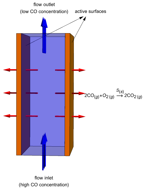
This study is to simulate mass transportation of molecules within a catalytic converter and its evolution in time. The catalytic converter modeled in this example consists of two parallel plates (active surfaces) with a catalyst on them. A gas containing molecules enters the domain from the bottom, flows across the reacting plates, and then exits the converter through the top. During this process the molecules near the plates are continuously oxidized into carbon dioxide:

In the Post-Processing section we will measure the converter performance by calculating the net reduction in the concentration: between the flow inlet and outlet :

For this the mean concentration at the boundary is computed with a boundary integration using NIntegrate:

The catalytic converter model is built and solved from time to . We will then determine when the system reaches its steady state.

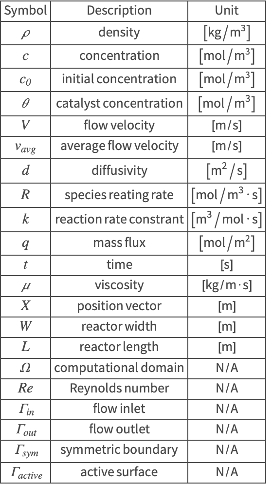
The symbols and corresponding units used here are summarized in the Nomenclature section.

Please refer to the information provided in "Mass Transport Tutorial" for a more general theoretical background for heat transfer analysis.

Load the finite element package.

Mass Transport Model

The conservative transport equation (1), which is derived from mass conservation, is used to solve for the concentration distribution in a mass transport model:

Here
is the concentration of the transported species ,
is the species diffusivity ,
is the velocity field of possible flow inside of the medium ,
is the mass production/consumption, the volumetric reacting rate of the species .

In this model the reaction of the carbon monoxide, , takes place on the active surfaces only, and will be modeled with a mass flux boundary condition. Since no other reaction occurs within the converter, the volumetric reacting rate is set to zero and the transport equation simplifies to:

Set up the model variables vars.

Set up the conservative model form.

Set up the diffusivity

of the carbon monoxide.

Domain

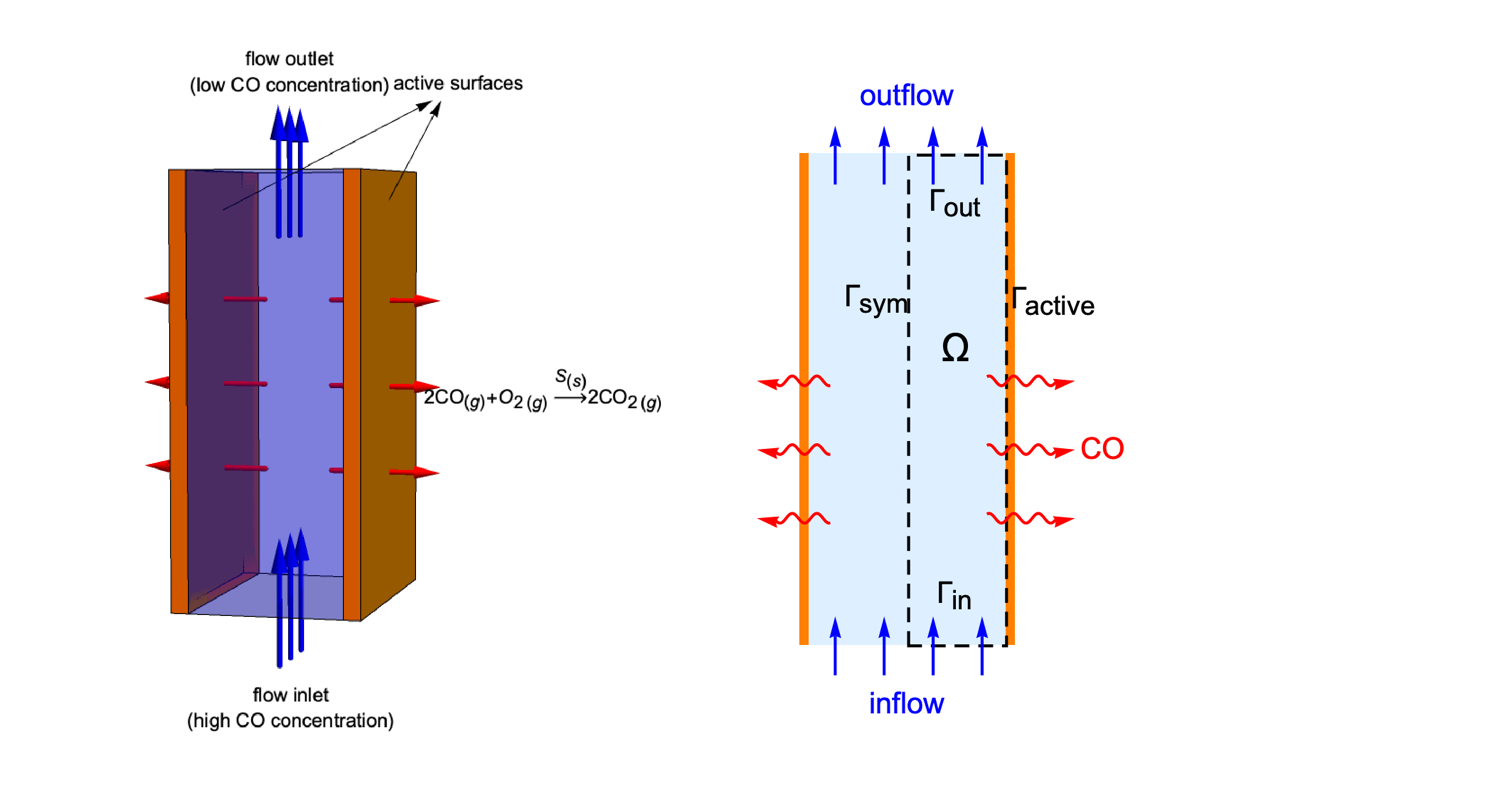
The catalytic converter model consists of two parallel reacting plates. If the depth of the plates is reasonably longer than its length and width, then the variation of concentration in the direction can be neglected. Therefore a two dimensional model is sufficient to represent the 3D reactor.

Due to the symmetry along the axis it is effective to only make use of the right half of the reactor as the simulation domain . Here and denote the flow inlet and flow outlet. The active surface and the symmetric boundary are symbolized as and , respectively.

Specify parameters of the geometry.

Define the 2D domain

Flow Regime

In this model the exhausted gas is flowing through the reactor at an average velocity of . To determine whether the gas flow is laminar or turbulent, we inspect the Reynolds number within the domain:

Here the density and the viscosity of the gas flow are given by and , respectively. The characteristic length is taken as the length of the reactor .

Evaluate the Reynolds number of the gas flow.

Empirically, the flow is considered as laminar when and as turbulent when .

Therefore, the flow velocity within the reactor can be determined by the analytical laminar profile:

Specify the flow velocity profile within the domain.

Initial and Boundary Conditions

At the beginning of the simulation, the carbon monoxide is uniformly distributed in the converter with an initial concentration .

Set up the initial condition of the concentration field.

There are four types of the boundary conditions involved in this mass transport model. At the flow inlet the concentration is held fixed at . There is an infinite supply of behind the inlet.

Set up a concentration boundary condition at the flow inlet

At the top boundary an outflow boundary condition is used to model the flow outlet where molecules are transported out of the domain.

Set up an outflow boundary condition at the flow outlet

On the active surface the carbon monoxide is absorbed and transformed by the catalyst , and can be modeled by a mass flux boundary condition.

Here the mass flux denotes the absorption rate of molecules, and is proportional to the its own concentration , the concentration of the remaining catalyst sites, , and the reaction rate constant :

Assuming that each carbon monoxide molecule occupies exactly one catalyst site during the reaction, then the concentration of remaining sites, , is equal to the difference between the total concentration of active sites, , and the number of sites occupied by the absorbed carbon monoxide:

Specify the mass flux of

molecules and set up a mass flux boundary condition on the active surface

A default symmetric boundary condition is implicitly applied on the symmetric boundary .

Solve the PDE Model

To analyze the transport of molecules and their evolution in time, the PDE model is solved from to .

Define the simulation end time.

Specify the mass transport PDE with the diffusivity

of the carbon monoxide.

Solve the PDE and monitor the time/memory usage.

Post-processing and Visualization

First, to inspect the effect of the catalytic converter we visualize the concentration evolving in time.

Set up a legend bar and ContourPlot options for the visualization.

Visualize the concentration field of the carbon monoxide.

See this note about improving the visual quality of the animation.

With the presence of the catalyst , molecules near the right boundary (active surface) are continuously absorbed and converted into carbon dioxide, resulting in a layer-like concentration field. The thickness of this concentration layer grows with time and reaches its steady state around .

Since the concentration has little variation outside this layer, it is known as the "reaction dead space". To minimize the reaction dead space and improve the overall converting effectiveness, the catalyst converter are often made in a shape of honeycombs rather than parallel plates.

To determine the exact time when the system reaches the steady state, we can use WhenEvent to check whether the concentration field has converged within the pre-defined threshold.

In this case we say the system is in steady state once the concentration derivative is below :

Take sampling points throughout the domain.

Set the threshold and detect the time required,

, to reach the steady state.

To see how the molecules vary in the flow direction, we can plot the concentration along the vertical line .

Inspect the

concentration along

at different time steps.

Note that the curves for , and are almost overlapping, which means the system has already reached it's steady state.

To measure the effectivity of the catalytic converter, the net reduction is calculated between the flow inlet and outlet . For this the mean concentration at the boundary is computed with a boundary integration: