


WhenEvent
Details and Options


- In NDSolve[eqns,…] the WhenEvent expressions are included in eqns and can be considered a part of the specification for the solution, especially for piecewise or hybrid systems.
- WhenEvent expressions can be used in NDSolve, NDSolveValue, ParametricNDSolve, ParametricNDSolveValue, DSolve, and DSolveValue.
- An event corresponds to a particular time
 crossed during the integration of eqns in NDSolve.
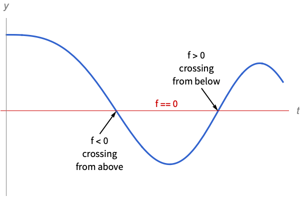
 - In cases where the event expression is given explicitly in terms of a function f of the solution such that the event becomes True at the roots of f, then WhenEvent uses a numerical root-finding procedure to determine an interval
 , where
  is the time where the function has a root. Examples of explicitly given events are:
 -
f0 the function f of the solution variables crosses zero f>0 f crosses zero from below f<0 f crosses zero from above Mod[t,  ]0
]0sample at regular intervals  in the time variable
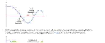
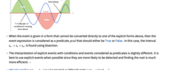
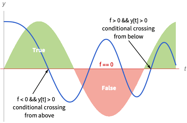
- With an explicit event expression ev, the event can be made conditional on a predicate pred using the form ev && pred. In this case, the event is only triggered if pred is True at the root of the event function.
- When the event is given in a form that cannot be converted directly to one of the explicit forms above, then the event expression is considered as a predicate pred that should either be True or False. In this case, the interval
 is found using bisection.
 - The interpretation of explicit events with conditions and events considered as predicates is slightly different. It is best to use explicit events when possible since they are more likely to be detected and finding the root is much more efficient. »
- WhenEvent[{event1,…},action] is treated as {WhenEvent[event1,action],…}.
- With WhenEvent[event,{action1,action2,…}], the actions are evaluated sequentially.
- The value from the evaluation of action is ignored by WhenEvent unless it has a special value that is used to affect NDSolve. The following special values are recognized:
-
"StopIntegration" stop integrating at  , return the solution
"RestartIntegration" restart the integration at 
"CrossDiscontinuity" integrate to  , extrapolate, and restart at
"CrossSlidingDiscontinuity" integrate to  , extrapolate and check sliding mode conditions, and restart at
"RemoveEvent" remove the event y[t]->val change the state variable y to val d[t]->"DiscontinuitySignature" change the discontinuity signature variable d - With WhenEvent[f==0,d->"DiscontinuitySignature"], the discontinuity is the surface f==0, and d must be a discrete variable that takes on values {-1, 0, 1} or {-1, 1} and is effectively set to Sign[f] for
 subsequent to the event.
 - WhenEvent has attribute HoldAll, so by default the event and action are only evaluated with variables assigned approximated values.
- WhenEvent can take the following options:
-
"DetectionMethod" Automatic the method to use for detecting an event "LocationMethod" Automatic the method to use for locating an event within a time step "IntegrateEvent" Automatic whether to integrate the event function "Priority" Automatic priority for actions of simultaneous events - Possible settings for "DetectionMethod" are:
-
Automatic automatically determine detection method "Sign" use a sign change "DerivativeSign" use sign change and time derivative "Interpolation" use interpolation of dense solution output - The "Sign" detection method has the least overhead, but may miss events in rapidly varying functions. The "Interpolation" detection method is more robust and may detect multiple events per step.
- Possible settings for "LocationMethod" are:
-
Automatic automatically determine location method "StepBegin" locate the event at the beginning of a step "StepEnd" locate the event at the end of a step "LinearInterpolation" linearly interpolate within a step "Brent" use Brent's root location within a step - Possible settings for "IntegrateEvent" are:
-
Automatic automatically determined False do not integrate the event function True integrate the event function - The settings for "Priority" can be any integer or Infinity. In the case of simultaneous events, the actions will be evaluated in sorted priority order.
Examples
open all close allScope (16)
Events (6)
Print the value of t whenever x[t] crosses 1/2:
Print the value of t whenever x[t] becomes greater than 1/2:
Print the value of t whenever x[t] becomes less than 1/2:
Sample the solution at regular time intervals ![]() :
:
Specify several events in a list to trigger an event when any of them occur:
Use an event ![]() with the condition
with the condition ![]() to detect crossings of the positive
to detect crossings of the positive ![]() axis:
axis:
In general, the event can be any expression that can be tested for becoming True:
Trigger an event to stop integration when a button is clicked:
If the Stop button is clicked soon enough, the integration will be terminated before ![]() :
:
Actions (9)
Specify several actions in a list to be executed in consecutive order:
Use "StopIntegration" to end the solution at an event:
Use "RemoveEvent" to remove an event after the first occurrence:
Remove an event after the third occurrence:
Use "RestartIntegration" to force restarting integration after an event:
A better way to handle this change is to use a discrete state variable a[t]:
Rules can be used to modify DependentVariables or DiscreteVariables:
Use "CrossDiscontinuity" to manage a discontinuity crossing:
Use "CrossSlidingDiscontinuity" to indicate that Filippov continuation can be used:
Use DiscreteVariables and "DiscontinuitySignature" to efficiently cross a discontinuity:
In the Filippov sliding mode case, the "DiscontinuitySignature" will be 0:
Options (11)
"DetectionMethod" (3)
The default event detection method is "Sign", which checks for sign changes between steps:
"Sign" can miss events if there is an even number of crossings between steps:
"DerivativeSign" halves the step if the sign is the same, but the derivative sign changes:
For rapidly varying event functions, use the "Interpolation" method to locate the events:
"LocationMethod" (3)
"IntegrateEvent" (2)
When an event function is varying more rapidly than the solution, crossings may be missed:
Plot the event function between ![]() and
and ![]() , with the time steps and crossings found:
, with the time steps and crossings found:
With "IntegrateEvent"->True, the steps taken are much smaller:
Define a function for comparing event-detection performance:
With "DetectionMethod"->"Interpolation", the event is integrated by default for robustness:
Applications (21)
Bouncing Balls (3)
Model a ball bouncing down steps:
Plot the ball's kinetic, potential, and total energy:
Model 20 bouncing balls dropped simultaneously from different heights:
In a square box, model a ball that changes direction upon impact with the side walls:
With an irrational initial velocity vector, there are no longer periodic solutions:
Optimization (1)
Crossing Detection (3)
Mark the points of arc length 1 for a parametric curve:
Mark the points where a parametric solution enters or leaves an annular region:
Mark only the points where a parametric solution leaves a region:
Mark only the points where a parametric solution enters a region:
Mark the points where the solution enters or leaves a region:
Hybrid Dynamical Systems (3)
Each time a linear oscillator solution crosses the negative ![]() axis, reflect it across the
axis, reflect it across the ![]() axis:
axis:
The solution of this reset oscillator exhibits chaotic behavior:
Plot the solution on the negative ![]() axis with a histogram of the reflection points:
axis with a histogram of the reflection points:
Model a one-degree-of-freedom impact oscillator with sinusoidal forcing:
Model a damped oscillator that gets a kick at regular time intervals:
The trajectory eventually settles into a consistent orbit:
Use the same oscillator, but give a random kick at regular time intervals:
Friction Models (1)
Model a block on a moving conveyor belt anchored to a wall by a spring using different models for the friction force ![]() , including viscous, Coulomb, Stribeck, and static. Compare positions and velocities for the different models:
, including viscous, Coulomb, Stribeck, and static. Compare positions and velocities for the different models:
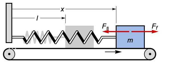
Newton's equation for the block:
Viscous friction is proportional to the relative velocity ![]() :
:
The block stabilizes just above the spring's natural length of 1:
Coulomb friction is proportional to the sign of relative velocity ![]() :
:
The block moves with the belt until the spring force is strong enough:
Stribeck friction is a refined Coulomb friction ![]() :
:
The variation at low velocities is slightly reduced:
Static friction holds the block in place until the spring force exceeds some value μ depending on roughness of surfaces. Use the discrete variable stuck set to 1 when the block is stuck and 0 otherwise:
Check whether the spring force is smaller than μ, and if the block is not moving relative to the belt:
The block repeatedly sticks to the belt, then slips away due to the spring force:
Power Electronics (4)
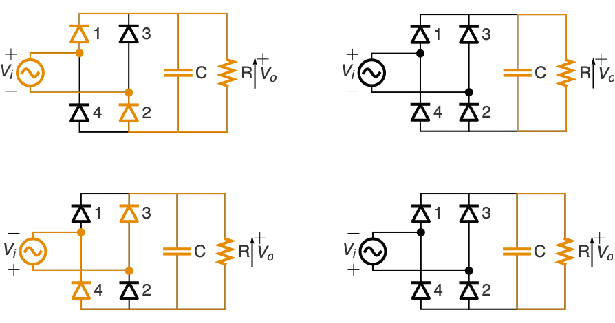
Model an AC-to-DC full wave rectifier with four diodes and a capacitor for smoothing the output:
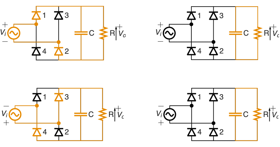
The input voltage vi and rectified voltage vr:
When vr increases, vo[t]=vr[t]; it charges the capacitor and supplies current to the load. When vr starts to decrease (vr'[t]<0), the capacitor discharges through the load and the output voltage follows vo'[t]=vo[t]/c r :
Plot the smoothened capacitor output voltage:
Model a DC-to-DC buck converter from input voltage level vi to desired output voltage level vd using a pulse-width modulated feedback control q[t]:

Use Kirchhoff's laws to get a model for the circuit above:
The control signal q[t] will switch the transistor on for a fraction vd/vi of each period τ:
Buck from a higher voltage vi=24 to a lower voltage vd=16:
Model a DC-to-DC boost converter from input voltage level vi to desired output voltage level vd using a pulse-width modulated feedback control q[t]:
Use Kirchhoff's laws to get a model for the circuit above:
The control signal q[t] will switch the transistor on for a fraction vi/vd of each period τ:
Boost from a lower voltage vi=24 to a higher voltage vd=36:
Model a DC-to-DC buck-boost converter from input voltage level vi to desired output voltage level vo using a pulse-width modulated feedback control q[t]:

Use Kirchhoff's laws to get a model for the circuit above:
The control signal q[t] will switch the transistor on for a fraction vd/(vi+vd) of each period:
Digital Control (5)
Simulate the system ![]() stabilized with a discrete-time controller
stabilized with a discrete-time controller ![]() :
:
Control a double integrator using a dead-beat discrete-time controller:
Use a dead-beat digital feedback controller ![]() :
:
Model the position of a moving body with 1 kg mass:
Use a sampled proportional-derivative (PD) controller to keep the position constant:
Design a discrete-time controller for the plant with state equations ![]() ,
, ![]() and output
and output ![]() and simulate the closed-loop system:
and simulate the closed-loop system:
Design a continuous-time controller by using a state estimator and state feedback:
Get a discrete-time controller by sampling with sample time ![]() :
:
Use the discrete-time controller:
Simulate the closed-loop system with the controller and plant together:
Model a pendulum at angle θ anchored to a moving cart at position x undergoing a horizontal force f:
Design a controller to stabilize the pendulum about the unstable vertical fixed point:
Use WhenEvent to apply the feedback at regular sample times:
The pendulum's angle is quickly stabilized in the inverted position (![]() ):
):
PDE Models (1)
Model thermostat-controlled heat generation in a room with three insulated walls and a glass front subject to the outside temperature:
A heater load is ramped up or down at an event. The factor of 20 specifies the slope of the transition:
Visualize the heater at an arbitrary event time of 10:
Note that there is an overlap in the up and down phases. This prevents them from continuously jumping between the two states, much like a real controller would.
The PDE models heat diffusion through air while generating heat inside a circle ![]() and losing heat through the glass window:
and losing heat through the glass window:
If the thermostat at position ![]() measures a temperature below/above a trigger, and if the discrete variable
measures a temperature below/above a trigger, and if the discrete variable ![]() changed, the heater is switched on/off:
changed, the heater is switched on/off:
Monitor the time integration of the PDE with initial condition equal to the outside temperature:
Visualize the temperature measured at the thermostat, the outside temperature, and the triggers for the heater. A blue background is shown where the heater is on:
Inspect the time steps taken during the integration and note how NDSolveValue adjusted the time step size as needed during events:
Properties & Relations (2)
NDSolve will try to automatically set up a WhenEvent event to handle a discontinuity in ![]() :
:
After automatic discontinuity processing, the following equivalent problem is solved:
If ![]() is a black-box function, NDSolve cannot automatically process the discontinuity:
is a black-box function, NDSolve cannot automatically process the discontinuity:
In this case, proper discontinuity handling can be achieved by adding a WhenEvent:
Alternatively, the discontinuity can be crossed using "CrossSlidingDiscontinuity":
Possible Issues (6)
Event Interpretation (1)
Events given explicitly with conditions have a slightly different interpretation than a single predicate:
WhenEvent cannot find an explicit root function, so the event occurs when pred becomes True:
When an explicit function (![]() ) is given, the event is considered as the root
) is given, the event is considered as the root ![]() but is conditional on the predicate (
but is conditional on the predicate (![]() ) that is False at
) that is False at ![]() , so it is never triggered:
, so it is never triggered:
Show the solution trajectory and the event location with the background colored green where the condition is True and red where it is False:
When an explicit function (![]() ) is given, the event is considered as the root
) is given, the event is considered as the root ![]() :
:
Show the solution trajectory and the event location with the background colored green where the condition is True and red where it is False:
Event Detection (2)
Arbitrarily Close Events (1)
Some systems admit an infinite number of events in a finite span of time:
Eventually, an event is not detected:
Tightening the tolerances for locating events improves detection:
Events will not be detected if they are closer than this:
With detection by interpolation, event detection can be further improved:
The gap between the last two events is very close to this limit:
Stop the integration automatically before events are missed:
Events are detected up to the point at which integration is stopped:
Increasing the working precision allows detection of events on a finer time scale:
Related Guides
Text
Wolfram Research (2012), WhenEvent, Wolfram Language function, https://reference.wolfram.com/language/ref/WhenEvent.html (updated 2014).
CMS
Wolfram Language. 2012. "WhenEvent." Wolfram Language & System Documentation Center. Wolfram Research. Last Modified 2014. https://reference.wolfram.com/language/ref/WhenEvent.html.
APA
Wolfram Language. (2012). WhenEvent. Wolfram Language & System Documentation Center. Retrieved from https://reference.wolfram.com/language/ref/WhenEvent.html
BibTeX
@misc{reference.wolfram_2025_whenevent, author="Wolfram Research", title="{WhenEvent}", year="2014", howpublished="\url{https://reference.wolfram.com/language/ref/WhenEvent.html}", note=[Accessed: 05-May-2026]}
BibLaTeX
@online{reference.wolfram_2025_whenevent, organization={Wolfram Research}, title={WhenEvent}, year={2014}, url={https://reference.wolfram.com/language/ref/WhenEvent.html}, note=[Accessed: 05-May-2026]}