Mass Transport
| Contents | Appendix |
| Introduction | Nomenclature |
| Mass Balance Equation | References |
| Boundary Conditions in Mass Transport |
Contents
Introduction
This tutorial gives an introduction to modeling mass transport of diluted species. Equations and boundary conditions that are relevant for performing mass transport analysis are derived and explained.
Mass transport is a discipline of chemical engineering that is concerned with the movement of chemical species. The two mechanisms of mass transport are mass diffusion and mass convection. The driving force behind a mass diffusion is the difference in a species concentration at different locations. Mass convection, on the other hand, only occurs when species are transported in a moving fluid medium. The combination of these two mechanisms leads to changes in the species concentration field over time and is modeled with a mass balance equation.
The modeling process results in a partial differential equation (PDE) that can be solved with NDSolve. Furthermore, in this tutorial, different types of mass transport boundary conditions are introduced. For the boundary conditions given, the modeling of various real-world chemical species interactions is shown.
This tutorial provides an introduction overview of how to model mass transport. The focus is to present simple yet illustrative examples. Extended examples that show industrial applications of mass transport modeling can be found in the "Mass Transfer Model Collection".
Many of the animations of the simulation results shown in this tutorial are generated with a call to Rasterize. This is to reduce the disk space required. The downside is that the visual quality of the animations will not be as crisp as without it. To obtain high-quality graphics, remove or comment out the call to Rasterize.
(*frames=Rasterize[#1,"Image",ImageResolution->35]&/@frames;*)The symbols and corresponding units used throughout this tutorial are summarized in the Nomenclature section.
Needs["NDSolve`FEM`"]Mass Balance Equation
The following sections start with an introduction of the mass balance equation, followed by a derivation of the equation and examples of how it is mapped to the Wolfram Language.
Mass Balance Equation Introduction
There are two different formulations that can be used to model the transport of chemical species through mass diffusion and mass convection. These are the conservative and non-conservative forms of the mass balance equation:

The dependent variable in the mass balance equation is the species concentration ![]() , which varies with time
, which varies with time ![]() and position
and position ![]() . The partial differential equation (PDE) model describes how chemical species are transported over time in a solid or fluid medium.
. The partial differential equation (PDE) model describes how chemical species are transported over time in a solid or fluid medium.
Typically, the non-conservative formulation is appropriate for incompressible fluids where the concentration field ![]() is expected to be smooth. The derivation in the section Mass Balance Equation Derivation will help explain why this is the case.
is expected to be smooth. The derivation in the section Mass Balance Equation Derivation will help explain why this is the case.
Besides the time derivative part, both PDEs are made up of several components. First and foremost, there is a diffusive term: ![]() with a diffusion coefficient
with a diffusion coefficient ![]() , which is also known as the species diffusivity. In some cases, the diffusion coefficient may depend on other properties, such as a temperature
, which is also known as the species diffusivity. In some cases, the diffusion coefficient may depend on other properties, such as a temperature ![]() and the concentration
and the concentration ![]() itself making the equation nonlinear. The details of variable diffusion coefficients will be discussed later in the section Variable Mass Diffusion Coefficient.
itself making the equation nonlinear. The details of variable diffusion coefficients will be discussed later in the section Variable Mass Diffusion Coefficient.
The second component is a convective term. In the conservative formulation, the convective term is ![]() . In the non-conservative formulation, the convective term is
. In the non-conservative formulation, the convective term is ![]() . The difference between the conservative and the non-conservative forms is explained in the section Mass Balance Equation Derivation. In either case, this term is only present if mass transport occurs in a fluid medium with a fluid flow velocity
. The difference between the conservative and the non-conservative forms is explained in the section Mass Balance Equation Derivation. In either case, this term is only present if mass transport occurs in a fluid medium with a fluid flow velocity ![]() . If the simulation medium is a solid, then this term is zero, regardless of which formulation is made use of.
. If the simulation medium is a solid, then this term is zero, regardless of which formulation is made use of.
Contrary to the convective term, the diffusive term may be present if the medium is solid or fluidic.
The term ![]() denotes a mass production or consumption rate of chemical species, typically due to a chemical reaction. This will be further explained in the Mass Transport with Chemical Reaction section.
denotes a mass production or consumption rate of chemical species, typically due to a chemical reaction. This will be further explained in the Mass Transport with Chemical Reaction section.
Mass Balance Equation Derivation
To derive the mass balance equation, start from the law of mass conservation. In a system, the total mass change must be equal to net mass formation minus the net mass outflow flow. A mass balance can then be expressed as:
To formulate the mass balance equation, the mass of a chemical species is balanced within a unit volume domain ![]() . The mass balance is based on the concentration
. The mass balance is based on the concentration ![]() of the species, which denotes the amount of species per unit volume measured in moles. The molar concentration
of the species, which denotes the amount of species per unit volume measured in moles. The molar concentration ![]() could be converted to a mass concentration
could be converted to a mass concentration ![]() by:
by:
where ![]() is the amount of the species in moles,
is the amount of the species in moles, ![]() is the volume of the domain,
is the volume of the domain, ![]() is the mass of the species, and
is the mass of the species, and ![]() is the molar mass, which is the mass per unit mole of the species.
is the molar mass, which is the mass per unit mole of the species.

In the above graphic, ![]() is the concentration and
is the concentration and ![]() is the area of the domain. The total mass within the control area is then equal to
is the area of the domain. The total mass within the control area is then equal to ![]() . The term
. The term ![]() denotes the net rate of mass formation due to chemical reactions inside the domain
denotes the net rate of mass formation due to chemical reactions inside the domain ![]() . The net mass flux
. The net mass flux ![]() represents the net rate of mass flow that exits through the boundaries.
represents the net rate of mass flow that exits through the boundaries.
The above consideration in 2D is valid in any dimension; for example, in a 3D domain, the concentration ![]() is given in
is given in ![]() and the volume in
and the volume in ![]() .
.
The unit of the mass flux ![]() through the boundary depends on the dimensionality of the boundary. In a 3D domain, the boundary is represented by 2D surfaces, and the mass flux
through the boundary depends on the dimensionality of the boundary. In a 3D domain, the boundary is represented by 2D surfaces, and the mass flux ![]() has a unit of
has a unit of ![]() . In a 2D domain, however, the boundary is made up of 1D lines, which makes the unit of
. In a 2D domain, however, the boundary is made up of 1D lines, which makes the unit of ![]() become
become ![]() . In 1D, the boundary is represented by a dimensionless point, and the heat flux
. In 1D, the boundary is represented by a dimensionless point, and the heat flux ![]() has a unit of
has a unit of ![]() .
.
The mass conservation within the domain ![]() can be described by the following equation:
can be described by the following equation:
That is, the rate of the mass change ![]() is equal to the net rate of mass formation
is equal to the net rate of mass formation ![]() inside the domain minus the net mass flux
inside the domain minus the net mass flux ![]() that exits the domain.
that exits the domain.
Here the mass flux ![]() can be divided into two parts: a diffusive mass flux
can be divided into two parts: a diffusive mass flux ![]() and a convection mass flux
and a convection mass flux ![]() . The diffusion flux describes the mass transport due to a concentration gradient in the mass species concentration and is proportional to its diffusivity
. The diffusion flux describes the mass transport due to a concentration gradient in the mass species concentration and is proportional to its diffusivity ![]() :
:
Equation (1) is also known as Fick's law of diffusion [2]. The minus sign states that the mass diffusion is in the direction of decreasing concentration.
The convection flux denotes the mass transported by a flow of the medium and is proportional to the flow velocity ![]() :
:
If the mass transport occurs in a solid medium, then, because a solid can not have an internal velocity field ![]() by definition, the convection term is set to
by definition, the convection term is set to ![]() .
.
Inserting (3) and (4) into the mass conservation equation (5) yields the conservative mass transport model.
When expressing (6) in the coefficient form of PDEs: ![]() , one has to be careful about the sign of the convection term
, one has to be careful about the sign of the convection term ![]() .
.
Equation (7) is known as the conservative mass balance equation since the convective mass flux term, ![]() , and with it the flow velocity
, and with it the flow velocity ![]() is inside of the divergence operator.
is inside of the divergence operator.
To obtain the non-conservative formulation equation (8) is expanded using the chain rule:
This results in the terms ![]() and
and ![]() . For an incompressible fluid, the divergence of the flow velocity is zero (
. For an incompressible fluid, the divergence of the flow velocity is zero (![]() ) by definition, and thus the term
) by definition, and thus the term ![]() equals zero, resulting in the non-conservative mass balance equation (9).
equals zero, resulting in the non-conservative mass balance equation (9).
If possible, it is recommended to use the non-conservative form for incompressible fluids when solving mass transport models. The two main reasons are:
- The removal of the term
 ensures that the incompressible flow field
  will not induce any nonphysical mass production or consumption into the source term
  .
.
- The mass convection term (10) is outside of the divergence operator, which prevents the growth of spurious oscillation of the solution field [11] and makes the PDE model more stable and efficient to solve.
However, the non-conservative formulation is only applicable for incompressible fluids where the concentration field ![]() is expected to be smooth. For mass transport in a compressible medium, the conservative formulation (12) should be used instead. Note that when the fluid flow velocity is zero, both models simplify to the same PDE.
is expected to be smooth. For mass transport in a compressible medium, the conservative formulation (12) should be used instead. Note that when the fluid flow velocity is zero, both models simplify to the same PDE.
This tutorial focuses on incompressible fluid media, and the non-conservative mass balance equation (13) will be used as the default PDE setup for the mass transport model. However, the later section Boundary Conditions in Mass Transport presents the boundary condition setup for both the conservative and the non-conservative formulations.
The mass balance equation may also be expressed in cylindrical and spherical coordinates. The details can be found in the appendix section Special Cases of the Mass Balance Equation.
The next section sets up the mass transport model function in the Wolfram Language.
Mass Transport Model Setup
The inputs needed for a mass transport model in Cartesian coordinates are
| the concentration variable | ||
| the spatial independent variables | ||
| a velocity field | ||
| the species diffusivity | ||
| the reaction rate (also known as the rate of mass formation) |
MassTransportPDEComponent[{c[x], {x}}, <|"DiffusionCoefficient" -> {{d}}, "MassConvectionVelocity" -> {Subscript[v, x]}, "MassSource" -> R|>]MassTransportPDEComponent[{c[x], {x}}, <|"DiffusionCoefficient" -> {{d}}, "MassConvectionVelocity" -> {Subscript[v, x]}, "MassSource" -> R, "ModelForm" -> "Conservative"|>]MassTransportPDEComponent[{c[t, x], t, {x}}, <|"DiffusionCoefficient" -> {{d}}, "MassConvectionVelocity" -> {Subscript[v, x]}, "MassSource" -> R|>]MassTransportPDEComponent[{c[t, x], t, {x}}, <|"DiffusionCoefficient" -> {{d}}, "MassConvectionVelocity" -> {Subscript[v, x]}, "MassSource" -> R, "ModelForm" -> "Conservative"|>]Note that this model definition uses inactive PDE operators. The tutorial "Numerical Solution of Partial Differential Equations" has several sections that explain the use of inactive operators.
In the next few sections, the mass transport model will be discussed in more detail. Various types of the usage of the mass transport PDE will be presented with examples.
Initial Mass Transport Example
The purpose of the 2D stationary example below is to demonstrate a typical workflow of mass transport modeling.
For this, consider a parallel-plate reactor with a species ![]() solved in water. As the water flow passes through the reactor, part of the species
solved in water. As the water flow passes through the reactor, part of the species ![]() will be absorbed by the active surface located at the right side. The goal is to find the steady-state concentration field for the species
will be absorbed by the active surface located at the right side. The goal is to find the steady-state concentration field for the species ![]() within the reactor.
within the reactor.

To make the example concrete, use a width of ![]() and a height of
and a height of ![]() for the model domain
for the model domain ![]() , and set the absorption rate
, and set the absorption rate ![]() on the active surface at the right shown in light gray. The left-side wall shown in black is assumed to be impermeable by the species
on the active surface at the right shown in light gray. The left-side wall shown in black is assumed to be impermeable by the species ![]() and thus has no mass flux across it.
and thus has no mass flux across it.
Ω2D = Rectangle[{0, 0}, {0.2, 0.5}];vars = {c[x, y], {x, y}};
pars = <||>;This example uses an arbitrary mass diffusion coefficient.
pars["DiffusionCoefficient"] = 10 ^ -4;In this example, the water is flowing through the reactor at an average velocity of ![]() . The flow velocity field
. The flow velocity field ![]() within the reactor is determined by the laminar profile:
within the reactor is determined by the laminar profile:

pars[Subscript[v, x]] = 0;
pars[Subscript[v, avg]] = 5 * 10^-3;
pars["MassConvectionVelocity"] = {Subscript[v, x], 2Subscript[v, avg] * (1 - ((x - 0.1/0.1))^2)}
Next, the boundary conditions at each boundary are set up. The details of setting up mass transfer boundary conditions will be explained in detail in the section Boundary Conditions in Mass Transport.
At the flow inlet, the species concentration is held fixed at ![]() , as if there is an infinite supply of the species
, as if there is an infinite supply of the species ![]() below the inlet.
below the inlet.
Subscript[Γ, in] = MassConcentrationCondition[y == 0, vars, pars, <|"MassConcentration" -> 1000|>]On the active surface, the species ![]() is continuously absorbed at a given rate of
is continuously absorbed at a given rate of ![]() . This is modeled by a mass flux boundary condition.
. This is modeled by a mass flux boundary condition.
Subscript[Γ, active] = MassFluxValue[x == 0.2, vars, pars, <|"MassFlux" -> -0.5, "BoundaryUnitNormal" -> {1, 0}|>]Since the left-side wall is impermeable by the species ![]() , an impermeable boundary condition is used to model the boundary where there is no mass flux across it.
, an impermeable boundary condition is used to model the boundary where there is no mass flux across it.
Subscript[Γ, left] = MassImpermeableBoundaryValue[x == 0, vars, pars, <|"BoundaryUnitNormal" -> {-1, 0}|>]A default outflow boundary condition is implicitly applied at the top boundary to model the flow outlet where the species ![]() is transported out of the domain.
is transported out of the domain.
Next, solve the mass transport PDE model with a prescribed flow field ![]() and an arbitrarily chosen species diffusivity of
and an arbitrarily chosen species diffusivity of ![]() .
.
cfun = NDSolveValue[{MassTransportPDEComponent[vars, pars] == Subscript[Γ, active] + Subscript[Γ, left], Subscript[Γ, in]}, c, {x, y}∈Ω2D];Note that the argument "NoReaction" is used to denote that there is no internal reaction within the domain.
Legended[ContourPlot[cfun[x, y], {x, y}∈Ω2D, ...], BarLegend[...]]In this example, the species ![]() is exclusively absorbed on the active surface at the right boundary at a rate of
is exclusively absorbed on the active surface at the right boundary at a rate of ![]() , resulting in a layer-like concentration field.
, resulting in a layer-like concentration field.
The Catalytic Converter application model is a time-dependent mass transport mode.
Mass Transport with a Chemical Reaction
In the previous section, the chemical species did not undergo a chemical reaction. In the following section, the modeling of chemical reactions is explained.
The term ![]() in the mass balance equations (14) and (15) is used to model a mass formation (
in the mass balance equations (14) and (15) is used to model a mass formation (![]() ) or consumption rate (
) or consumption rate (![]() ) within the domain. Typical phenomena that lead to a mass formation or consumption are chemical reactions. As an example, consider the following 2D transient model:
) within the domain. Typical phenomena that lead to a mass formation or consumption are chemical reactions. As an example, consider the following 2D transient model:

The model domain ![]() has a internal rectangular region
has a internal rectangular region ![]() where an unimolecular reaction occurs. A unimolecular reaction happens when a chemical species
where an unimolecular reaction occurs. A unimolecular reaction happens when a chemical species ![]() undergoes a self-transformation into a single product
undergoes a self-transformation into a single product ![]() :
:
This example assumes the reaction to be a first-order reaction [16]; that is, the mass consumption rate ![]() of the reactant
of the reactant ![]() will be linearly proportional to the concentration
will be linearly proportional to the concentration ![]() of the reactant itself:
of the reactant itself:
Here, ![]() is the reaction rate constant and has a unit of
is the reaction rate constant and has a unit of ![]() . For most chemical reactions, the rate constant
. For most chemical reactions, the rate constant ![]() is temperature dependent and can be computed by the Arrhenius equation [17]. In this example, however, a constant
is temperature dependent and can be computed by the Arrhenius equation [17]. In this example, however, a constant ![]() is chosen for the sake of simplicity.
is chosen for the sake of simplicity.
Typically, applications where the reaction rate ![]() is temperature dependent are modeled as coupled equations where a heat equation is linked with a mass transport equation. An example of the setup of and modeling with a temperature-dependent reaction rate
is temperature dependent are modeled as coupled equations where a heat equation is linked with a mass transport equation. An example of the setup of and modeling with a temperature-dependent reaction rate ![]() can be found in the multiphysics application model Thermal Decomposition.
can be found in the multiphysics application model Thermal Decomposition.
Ω2D = Rectangle[];
Subscript[Ω2D, reaction] = Rectangle[{4 / 10, 45 / 100}, {6 / 10, 55 / 100}];vars = {c[t, x, y], t, {x, y}};
pars = <|"DiffusionCoefficient" -> 0.001|>;pars["MassReactionRate"] = If[RegionMember[Subscript[Ω2D, reaction]][{x, y}], 1, 0]Note that by using exact numbers for the region, the region membership test is simplified to an If statement.
To highlight the effect of the chemical reaction, assume that there is no moving flow within the domain, which means that the mass transport is by diffusion only.
pde = {MassTransportPDEComponent[vars, pars] == 0, c[0, x, y] == 1000};cfun = NDSolveValue[pde, c, {t, 0, 100}, {x, y}∈Rectangle[]];nframes = 30;
frames = Table[Show[Legended[ContourPlot[cfun[t, x, y], {x, y}∈Ω2D, ...], BarLegend[...]], Graphics[...]], {t, 0, 100, 100 / nframes}];
frames = Rasterize[#1, "Image", ImageResolution -> 80]& /@ frames;
ListAnimate[frames, SaveDefinitions -> True]See this note about improving the visual quality of the animation.
The species ![]() has an initial concentration field
has an initial concentration field ![]() of
of ![]() and is gradually consumed by the reaction within the region
and is gradually consumed by the reaction within the region ![]() . The excess species
. The excess species ![]() outside the region
outside the region ![]() then fills in by diffusion due to the concentration gradient, which brings down the overall concentration within the model domain.
then fills in by diffusion due to the concentration gradient, which brings down the overall concentration within the model domain.
An application example that shows a more evolved reaction model is given in the Microscale Simulation of Catalyst Deactivation model. A further model is the Gas Absorption at Liquid Surface model.
Anisotropic and Orthotropic Mass Diffusion
In previous sections, the assumption was that the species is transported in an isotropic medium; that is, the rate of the diffusive mass transfer is independent of its direction and given by the same concentration gradient ![]() . In reality, however, a medium may be anisotropic. Anisotropic diffusion means that the species diffuses in different directions with a different rate. Orthotropic diffusion is a special case of anisotropic mass diffusion that will be described below. Anisotropic behavior can be found all the way from natural products to sophisticated composite materials and as such, is an important phenomenon to be able to model.
. In reality, however, a medium may be anisotropic. Anisotropic diffusion means that the species diffuses in different directions with a different rate. Orthotropic diffusion is a special case of anisotropic mass diffusion that will be described below. Anisotropic behavior can be found all the way from natural products to sophisticated composite materials and as such, is an important phenomenon to be able to model.
Since the species diffusivity ![]() varies in different directions, the diffusion flux term (18) is then rewritten as:
varies in different directions, the diffusion flux term (18) is then rewritten as:
![]() is the diffusivity tensor.
is the diffusivity tensor. ![]() and
and ![]() are called the principle diffusion coefficients and off-diagonal diffusion coefficients, respectively.
are called the principle diffusion coefficients and off-diagonal diffusion coefficients, respectively.
With orthotropic diffusion, the species diffusivity of a material is symmetric but distinct along the principal directions ![]() ,
, ![]() and
and ![]() , such as shown in the graphics below. All the off-diagonal diffusion coefficients are zero. This behavior can be seen, for example, in fiber composite materials. Then the diffusion tensor becomes:
, such as shown in the graphics below. All the off-diagonal diffusion coefficients are zero. This behavior can be seen, for example, in fiber composite materials. Then the diffusion tensor becomes:
As an example, consider a 2D composite material with a layered-like structure. The initial concentration of the species can be described by a Gaussian bell shape centered at ![]() . The species then gradually diffuses throughout the entire domain.
. The species then gradually diffuses throughout the entire domain.

The illustration above depicts the orthotropic case where the species diffuses slower in the vertical direction, where it passes across the internal boundaries of the layered structure shown as gray lines. The diffusivity tensor can be described by:
Subscript[d, orthotropic] = {{Subscript[d, xx], 0}, {0, Subscript[d, yy]}} /. {Subscript[d, xx] -> 10 ^ -3, Subscript[d, yy] -> 10 ^ -4};ics = {c[0, x, y] == 1000 * Exp[-((x - 1 / 2) ^ 2 + (y - 1 / 2) ^ 2) / 0.01]};pde = {MassTransportPDEComponent[{c[t, x, y], t, {x, y}}, <|"DiffusionCoefficient" -> Subscript[d, orthotropic]|>] == 0, ics};
cfun = NDSolveValue[pde, c, {t, 0, 10}, {x, y}∈Rectangle[]];nframes = 30;
frames = Table[Show[Legended[ContourPlot[cfun[t, x, y], {x, y}∈Rectangle[], ...], BarLegend[...]]], {t, 0, 10, 10 / nframes}];
frames = Rasterize[#1, "Image", ImageResolution -> 80]& /@ frames;
ListAnimate[frames, SaveDefinitions -> True]See this note about improving the visual quality of the animation.
The species is transported faster in the horizontal direction, resulting in a higher concentration zone within the band between ![]() .
.
Variable Mass Diffusion Coefficient
In the preceding sections, the assumption was that the mass diffusion coefficient and hence the species diffusivity are either a constant scalar ![]() for an isotropic medium or a constant tensor
for an isotropic medium or a constant tensor ![]() for an anisotropic medium. In reality, however, the diffusivity might change significantly with temperature
for an anisotropic medium. In reality, however, the diffusivity might change significantly with temperature ![]() and the species concentration
and the species concentration ![]() . Both phenomena will be examined in turn.
. Both phenomena will be examined in turn.
Temperature dependence of the diffusion coefficient
When modeling mass transport in a medium with a nonuniform temperature field, it is better to account for the temperature dependence of the diffusion coefficient ![]() . As a starting model, the diffusion coefficient can be predicted by Arrhenius's equation:
. As a starting model, the diffusion coefficient can be predicted by Arrhenius's equation:
![]() is the species diffusivity
is the species diffusivity ![]() ,
,![]() is the maximum species diffusivity at infinite temperature
is the maximum species diffusivity at infinite temperature ![]() ,
,![]() is the absolute temperature
is the absolute temperature ![]() ,
,![]() is the activation energy for diffusion
is the activation energy for diffusion ![]() ,
,![]() is the gas constant
is the gas constant ![]() .
.
The exponential form of this relation means that the species diffusivity ![]() can grow quickly with temperature
can grow quickly with temperature ![]() .
.
As an example, consider a 1D domain ![]() with a prescribed temperature field increase from left to right as
with a prescribed temperature field increase from left to right as ![]() .
.
pars = <|e -> 10 ^ 4, Subscript[d, 0] -> 0.01, Subscript[R, g] -> Quantity["MolarGasConstant"]|>;pars["DiffusionCoefficient"] = Subscript[d, 0] Exp[-(e/Subscript[R, g] * (200 + 800x))];At time ![]() , the species is confined around the center and can be described by a Gaussian distribution.
, the species is confined around the center and can be described by a Gaussian distribution.
ics = {c[0, x] == 1000 * Exp[-(x - 1 / 2) ^ 2 / 0.01]};pde = {MassTransportPDEComponent[{c[t, x], t, {x}}, pars] == 0, ics};
cfun = NDSolveValue[pde, c, {t, 0, 100}, {x, 0, 1}];nframes = 30;
frames = Table[Show[Plot[cfun[t, x], {x, 0, 1}, ...],
Plot[...]], {t, 0, 100, 100 / nframes}];
ListAnimate[frames, Rule[...]]At time ![]() , the species is confined around the center and then gradually diffused throughout the domain. Note that the species diffused faster to the right side due to the higher temperature in that region.
, the species is confined around the center and then gradually diffused throughout the domain. Note that the species diffused faster to the right side due to the higher temperature in that region.
In this example, the temperature field ![]() is prescribed. However, to solve a mass transport model with an unknown temperature field, a multiphysics model has to be constructed that couples a heat transfer model with a mass transport model. Such a coupled heat transfer mass transport multiphysics application model is shown in the model collection in the Thermal Decomposition example.
is prescribed. However, to solve a mass transport model with an unknown temperature field, a multiphysics model has to be constructed that couples a heat transfer model with a mass transport model. Such a coupled heat transfer mass transport multiphysics application model is shown in the model collection in the Thermal Decomposition example.
Concentration dependence of the diffusion coefficient
For some mass transport applications such as drug delivery in blood and pollutants emission in air, the transported species may have unique interaction with the molecules of the medium [19, 20]. In such cases, the diffusion coefficient ![]() will be affected by the concentration field
will be affected by the concentration field ![]() of the transported species, leading to a nonlinear mass balance equation. The non-conservative nonlinear mass balance equation is given as:
of the transported species, leading to a nonlinear mass balance equation. The non-conservative nonlinear mass balance equation is given as:
The diffusion coefficient ![]() in the PDE model is now a function of the concentration
in the PDE model is now a function of the concentration ![]() itself. The expression of the nonlinear diffusion coefficient is usually determined experimentally and depends on the type of transported species and the medium.
itself. The expression of the nonlinear diffusion coefficient is usually determined experimentally and depends on the type of transported species and the medium.
As an example, consider a 1D mass transport model with an initial concentration field of ![]() , a reference diffusion coefficient
, a reference diffusion coefficient ![]() and a concentration-dependent diffusion coefficient
and a concentration-dependent diffusion coefficient ![]() . In this case, the species diffusivity
. In this case, the species diffusivity ![]() will increase with higher concentration
will increase with higher concentration ![]() .
.
To model the supply of species into the domain, a constant mass flux ![]() is applied at the left-hand boundary.
is applied at the left-hand boundary.
vars = {c[t, x], t, {x}};
pars = <|"DiffusionCoefficient" -> Subscript[d, 0] + 5 * 10 ^ -5 c[t, x], Subscript[d, 0] -> 0.01|>;Subscript[Γ, flux] = MassFluxValue[x == 0, vars, pars, <|"MassFlux" -> 5, "BoundaryUnitNormal" -> {-1}|>]pdeNonLinear = {MassTransportPDEComponent[vars, pars] == Subscript[Γ, flux], c[0, x] == 0};
cfunNonLinear = NDSolveValue[pdeNonLinear, c, {t, 0, 50}, {x, 0, 1}];To better understand the effects of the nonlinearity, compare to a linear mass transport PDE.
linearPars = pars;
linearPars["DiffusionCoefficient"] = Subscript[d, 0];
pdeLinear =
	{MassTransportPDEComponent[vars, linearPars] == Subscript[Γ, flux], c[0, x] == 0};
cfunLinear = NDSolveValue[pdeLinear, c, {t, 0, 50}, {x, 0, 1}];nframes = 30;
frames = Table[Show[Plot[{cfunLinear[t, x], cfunNonLinear[t, x]}, {x, -0.3, 1}, ...], Graphics[...]], {t, 0, 50, 50 / nframes}];
ListAnimate[frames, SaveDefinitions -> True]In both the linear and nonlinear model, the species entered the domain from the left with a constant mass flux ![]() . However, for the nonlinear model, the diffusion coefficient
. However, for the nonlinear model, the diffusion coefficient ![]() will increase with the concentration
will increase with the concentration ![]() , which further speeds up the mass transport and results in a flatter concentration field.
, which further speeds up the mass transport and results in a flatter concentration field.
Interphase Mass Transfer
In the preceding sections, the mass transfer by mass convection and mass diffusion in a single phase has been considered. However, there are many situations in nature where two different phases are in contact, and mass may be transported from one phase to the other. This process is known as interphase mass transfer.
Unlike the single-phase mass transfer where the concentration field is always continuous, the species concentration can jump at the interface between two states as follows:

Here ![]() and
and ![]() are the concentration of species dissolved in phase
are the concentration of species dissolved in phase ![]() and phase
and phase ![]() . The subscription
. The subscription ![]() denotes the species concentration at the interface between two phases.
denotes the species concentration at the interface between two phases.
A separate mass balance equation should be used to describe the species concentration ![]() in phase
in phase ![]() and
and ![]() in the phase
in the phase ![]() :
:
At the interface of two phases, the concentration may be discontinuous between ![]() and
and ![]() . The ratio
. The ratio ![]() is known as the equilibrium distribution coefficient
is known as the equilibrium distribution coefficient ![]() :
:
The coefficient ![]() depends on pressure, temperature and the chemical properties of the transported species, as well as the media of both phases. The value
depends on pressure, temperature and the chemical properties of the transported species, as well as the media of both phases. The value ![]() can be determined by experimental measurement [21].
can be determined by experimental measurement [21].
Assuming the molecules of species can penetrate quickly through the interface of two phases, the equilibrium condition (22) at the interface ![]() will be reached instantaneously and is satisfied at all times.
will be reached instantaneously and is satisfied at all times.
This assumption was first proposed by Whitman [23] as the two-resistance theory and is valid for most cases of the interphase mass transfer. However, in case a chemical reaction occurs at the interface, additional repulsive or attractive forces may act on the transported species, and then this assumption will no longer be valid.
Consider a 1D model where sulfur dioxide, ![]() , is transferred from air
, is transferred from air ![]() into water
into water ![]() . To model the interphase mass transfer, a thin interphase region will be defined between the two different phases, which will allow us to enforce the equilibrium condition (24) via a coupled fictitious mass sources and handle the discontinuity of the
. To model the interphase mass transfer, a thin interphase region will be defined between the two different phases, which will allow us to enforce the equilibrium condition (24) via a coupled fictitious mass sources and handle the discontinuity of the ![]() concentration at
concentration at ![]() .
.
Here the thickness ![]() of the interphase region is set to be
of the interphase region is set to be ![]() of the length
of the length ![]() of the domain. Note that if
of the domain. Note that if ![]() is set too small, a numerical instability may occur around the interface.
is set too small, a numerical instability may occur around the interface.
L = 1;
w = L / 100;
leftInterphasePos = L / 2 - w / 2;
rightInterphasePos = L / 2 + w / 2;
bmesh = ToBoundaryMesh["Coordinates" -> {{0}, {leftInterphasePos}, {rightInterphasePos}, {L}}, "BoundaryElements" -> {PointElement[{{1}, {2}, {3}, {4}}]}];
Next, a full element mesh with internal markers is defined to distinguish the gas, liquid and interphase regions. For clearer assignment of markers, an association is used.
regionMarker = <|"gas" -> 1, "interphase" -> 2, "liquid" -> 3|>;
mesh = ToElementMesh[bmesh, "RegionMarker" -> {
	{{0.2}, regionMarker["gas"]},
	{{0.5}, regionMarker["interphase"]},
{{0.8}, regionMarker["liquid"]}}];vars = {{Subscript[c, gas][t, x], Subscript[c, liquid][t, x]}, t, {x}};
pars = <||>;The diffusion coefficients of ![]() in the gas and liquid phases are given by
in the gas and liquid phases are given by ![]() and
and ![]() , respectively. Note that
, respectively. Note that ![]() and
and ![]() are only valid within the interphase region as well as their own phase.
are only valid within the interphase region as well as their own phase.
Subscript[d, gas] = If[ElementMarker == regionMarker["gas"] || ElementMarker == regionMarker["interphase"], 1 / 100, 0];
Subscript[d, liquid] = If[ElementMarker == regionMarker["liquid"] || ElementMarker == regionMarker["interphase"], 1 / 1000, 0];pars["DiffusionCoefficient"] = {{{{Subscript[d, gas]}}, 0}, {0, {{Subscript[d, liquid]}}}};To model the transfer of ![]() between two phases, add the coupling mass source terms
between two phases, add the coupling mass source terms ![]() and
and ![]() in the governing mass balance equation (25), leading to:
in the governing mass balance equation (25), leading to:
Here ![]() and
and ![]() are set at
are set at ![]() , so that the equilibrium condition (26)
, so that the equilibrium condition (26) ![]() can be enforced at the interface. In the equation,
can be enforced at the interface. In the equation, ![]() is the interphase mass transfer coefficient, and
is the interphase mass transfer coefficient, and ![]() is a switch that turns on
is a switch that turns on ![]() within the interphase region and off
within the interphase region and off ![]() otherwise.
otherwise.
σ = If[ElementMarker == regionMarker["interphase"], 1, 0];Based on the two-resistance theory mentioned above, the equilibrium at the interface is considered to be reached instantaneously and maintained at all times. This condition can be modeled by setting the mass transfer coefficient ![]() to be infinitely large.
to be infinitely large.
In practice, ![]() can be chosen to be greater than the species diffusivity
can be chosen to be greater than the species diffusivity ![]() and
and ![]() ) by several orders of magnitude.
) by several orders of magnitude.
k = 10^4 * (Subscript[d, gas] + Subscript[d, liquid]) /. {ElementMarker -> regionMarker["interphase"]};Subscript[Q, gas] = σ * k * (K Subscript[c, liquid][t, x] - Subscript[c, gas][t, x]);
Subscript[Q, liquid] = σ * k * (Subscript[c, gas][t, x] - K Subscript[c, liquid][t, x]);
pars["MassSource"] = {{Subscript[Q, gas]}, {Subscript[Q, liquid]}};Note that due to the mass conservation, the coupling source terms ![]() and
and ![]() have the same magnitude but opposite sign.
have the same magnitude but opposite sign.
To model the supply of ![]() into the domain, a constant mass flux
into the domain, a constant mass flux ![]() is applied at the left-hand boundary of the air region.
is applied at the left-hand boundary of the air region.
Subscript[Γ, flux] = MassFluxValue[x == 0, vars, pars, <|"MassFlux" -> {5, 0}, "BoundaryUnitNormal" -> {-1}|>];ics = {Subscript[c, gas][0, x] == 0, Subscript[c, liquid][0, x] == 0};pde = {MassTransportPDEComponent[vars, pars] == Subscript[Γ, flux], ics};To study the effect of the equilibrium coefficient ![]() on the interphase mass transfer, the PDE model is solved repetitively with ParametricNDSolveValue at
on the interphase mass transfer, the PDE model is solved repetitively with ParametricNDSolveValue at ![]() ,
, ![]() and
and ![]() :
:
cfun =
	ParametricNDSolveValue[pde, {Subscript[c, gas], Subscript[c, liquid]}, {t, 0, tend}, {x}∈mesh, {K}];
cfunTable = Table[cfun[K], {K, {0.5, 1, 1.5}}];Manipulate[Show[Plot[Piecewise[{
{cfunTable[[i, 1]][t, x], x ≤ leftInterphasePos}, {cfunTable[[i, 2]][t, x], x ≥ rightInterphasePos},
{Indeterminate, True}}], ...], Graphics[...]], ...]Note that as the equilibrium coefficient ![]() deviates from
deviates from ![]() , the jump between
, the jump between ![]() and
and ![]() increases.
increases.
The strategy presented in this section can also be applied in modeling mass transfer across a membrane. In that case, however, an additional repulsive force (i.e. surface resistance) may play a role, and the time for the membrane to reach the equilibrium condition (27) should also be considered. This can be done by selecting a ![]() value in (28) based on the surface resistance of the membrane.
value in (28) based on the surface resistance of the membrane.
Mass Source Types
Mass sources like volumetric, layer and point sources can be modeled in a similar fashion, as explained in the corresponding Heat Transfer model section.
Multiphysics Mass Transport
Mass transport can be combined with other fields of physics. What follows is a list of multiphysics application examples that make use of mass transport:
Boundary Conditions in Mass Transport
The most common boundary conditions in mass transport modeling can be modeled with DirichletCondition, NeumannValue and PeriodicBoundaryCondition and can be categorized in the following four types:
- Dirichlet-type boundary conditions. This type of boundary condition specifies the species concentration
 at the boundary and can be modeled with DirichletCondition.
- Neumann-type boundary conditions. This type of boundary condition specifies the mass flux
 at the boundary and can be modeled with NeumannValue.
- Robin-type boundary conditions. This type of boundary condition specifies the relation between the species concentration
 and its normal derivatives at the boundary and can modeled with a NeumannValue, since Robin-type boundary conditions are technically generalized Neumann boundary conditions.
- Periodic boundary conditions. This type of boundary condition specifies the species concentration
 at one part of the boundary to be the same at another part and can be modeled with PeriodicBoundaryCondition.
Under these four types, the following boundary conditions are introduced:
The following section describes several physical boundary conditions common in modeling mass transport and how they can be represented with the use of DirichletCondition, NeumannValue and PeriodicBoundaryCondition. For this purpose, the boundary condition currently discussed is always at the left-hand side of the example simulation domain. In some examples, additional boundary conditions are at the right-hand side to better demonstrate the behavior of the boundary condition at the left-hand side.
Note that the setup of Neumann-type boundary conditions will be slightly different between the conservative model and non-conservative model. The details of this difference are presented in the following section.
Neumann Values for Conservative and Non-conservative Models
In a previous section, the derivation and setup of the conservative and non-conservative mass transport model was presented. The difference of the model formulation has an impact on how Neumann-type boundary conditions are to be set up and what they mean.
With the conservative formulation, the NeumannValue specifies the boundary values for ![]() . With NeumannValue[val,X∈Γb], this means:
. With NeumannValue[val,X∈Γb], this means:
With the non-conservative formulation, the NeumannValue specifies the boundary values for ![]() . With NeumannValue[val,X∈Γb], this means:
. With NeumannValue[val,X∈Γb], this means:
Note that for the conservative formulation, the term: ![]() , which is the mass transported by a flow of the medium across the boundary, is also included in the Neumann value.
, which is the mass transported by a flow of the medium across the boundary, is also included in the Neumann value.
In some of the boundary conditions presented, the form of the Neumann value needs to changed. This means that, for example, a Neumann value in the conservative form like (29) will have to be transformed into:
Transformations of this sort pose a problem, as usually the normal ![]() in a Neumann formulation like the left side of (30) is never actually computed but replaced with the value of the right-hand side of (31). Once a normal
in a Neumann formulation like the left side of (30) is never actually computed but replaced with the value of the right-hand side of (31). Once a normal ![]() appears on the right-hand side of the equation, that value of the normal will have to be computed, and this is done automatically. If the boundary unit normal is simple, it can be specified with the model parameter "BoundaryUnitNormal". This may increase computational efficiency both in speed and memory usage.
appears on the right-hand side of the equation, that value of the normal will have to be computed, and this is done automatically. If the boundary unit normal is simple, it can be specified with the model parameter "BoundaryUnitNormal". This may increase computational efficiency both in speed and memory usage.
Before the mass transport boundary conditions for both the conservative model and non-conservative model are presented, some example model parameters are set up.
Model Parameter Setup
The following model parameters are made use of in the examples of mass transport boundary conditions. These parameters define the simulation domain ![]() and the simulation end time
and the simulation end time ![]() .
.
left = 0;
right = 1;
tend = 100;
Ω = Line[{{left}, {right}}];
In some examples, a smoothed step function ![]() will be used to prescribe a time profile for a transient parameter, such as, for example, the mass flux
will be used to prescribe a time profile for a transient parameter, such as, for example, the mass flux ![]() or the concentration
or the concentration ![]() on the boundary. The smoothed step function is defined as follows:
on the boundary. The smoothed step function is defined as follows:
Here, the minimum value and the maximum value of the function ![]() can reach are denoted by
can reach are denoted by ![]() and
and ![]() . The location of the step is controlled by
. The location of the step is controlled by ![]() , and the smoothed steepness is controlled by
, and the smoothed steepness is controlled by ![]() .
.
SmoothedStepFunction[fmin_, fmax_, ts_, m_] := Function[t, (fmin * Exp[ts * m] + fmax * Exp[m * t]) / (Exp[ts * m] + Exp[m * t])]Manipulate[Show[Plot[SmoothedStepFunction[fmin, fmax, ts, m][t], {t, 0, tend}, ...], Graphics[...]], ...]Concentration Boundary Condition
Purpose
The purpose of a concentration boundary condition is to set a specific species concentration on some part of the boundary.
Formulation
With a specified concentration ![]() on the boundary
on the boundary ![]() , the concentration boundary condition is given for both conservative and non-conservative models by:
, the concentration boundary condition is given for both conservative and non-conservative models by:
Since the concentration boundary condition is a Dirichlet-type condition and thus is not associated with the model equation, its formulation is the same for both the conservative model and non-conservative model.
MassConcentrationCondition[x∈Subscript[Γ, b], {c[t, x], t, x}, <|"MassConcentration" -> cs[t, x]|>]Derivation
A given species concentration ![]() is prescribed on a boundary. This prescribed concentration
is prescribed on a boundary. This prescribed concentration ![]() can either be a constant or time-dependent value and is set with a DirichletCondition in the mass transport PDE model.
can either be a constant or time-dependent value and is set with a DirichletCondition in the mass transport PDE model.
Example
To model, for example, the supply of a given species on a boundary, a transient species concentration ![]() can be set up at the left end. Note that a Neumann zero condition is implicitly applied at the right end as an outflow boundary.
can be set up at the left end. Note that a Neumann zero condition is implicitly applied at the right end as an outflow boundary.
Here a smoothed step function is used to describe the profile of the species concentration ![]() on the boundary from
on the boundary from ![]() to
to ![]() . The parameters
. The parameters ![]() and
and ![]() are arbitrarily chosen to simulate the supply of species from the boundary.
are arbitrarily chosen to simulate the supply of species from the boundary.
cMin = 0;
cMax = 1000;
ts = 25;
m = 0.25;cs = SmoothedStepFunction[cMin, cMax, ts, m];
Plot[cs[t], {t, 0, tend}, ...]Subscript[Γ, concentration] = MassConcentrationCondition[x == left, {c[t, x], t, x}, <|"MassConcentration" -> cs[t]|>]Next, set up the mass transport model with a flow field ![]() , an initial concentration field
, an initial concentration field ![]() and a diffusion coefficient
and a diffusion coefficient ![]() .
.
pde = {MassTransportPDEComponent[{c[t, x], t, {x}}, <|"DiffusionCoefficient" -> 0.01, "MassConvectionVelocity" -> {0.02}|>] == 0, Subscript[Γ, concentration], c[0, x] == 0};cfun = NDSolveValue[pde, c, {t, 0, tend}, x∈Ω];Visualization
nframes = 30;
frames = Table[Show[Plot[cfun[t, x], {x, -0.2, 1}, ...], Graphics[...]], {t, 0, tend, tend / nframes}];
ListAnimate[frames, SaveDefinitions -> True]
The simulation begins with an undisturbed domain where ![]() . As the concentration
. As the concentration ![]() increases at the left boundary, the excess species are then transported to the right and bring up the overall species concentration within the domain. The speed of the mass transport depends on the species diffusivity
increases at the left boundary, the excess species are then transported to the right and bring up the overall species concentration within the domain. The speed of the mass transport depends on the species diffusivity ![]() and the flow field.
and the flow field.
Outflow Boundary Condition
Purpose
If the mass transport occurs in a system where the flow velocity ![]() , then an outflow boundary condition is used to model an outlet where the species can leave the domain with the fluid flow.
, then an outflow boundary condition is used to model an outlet where the species can leave the domain with the fluid flow.
Formulation
When modeling mass transport in a fluid medium, the outflow boundary condition at the outlet ![]() is given by:
is given by:
MassOutflowValue[x∈Subscript[Γ, b], {c[t, x], t, {x}}, <|"MassConvectionVelocity" -> {V}, "ModelForm" -> "Conservative"|>]MassOutflowValue[x∈Subscript[Γ, b], {c[t, x], t, {x}}, <|"MassConvectionVelocity" -> {V}, "ModelForm" -> "NonConservative"|>]Note that for the non-conservative model, an outflow boundary condition is essentially a Neumann zero condition, which means it will be implicitly applied if no boundary condition is specified at a given boundary.
Derivation
When modeling mass transport with a fluid flow, the diffusion mass flux at the flow outlet is set to zero to ensure that the mass transferred at the outlet boundary is by mass convection only and the mass diffusion is ignored: ![]() .
.
With the non-conservative formulation, the NeumannValue[val,X∈Γb] specifies the boundary values (32): ![]() . So for
. So for ![]() , it is required that
, it is required that ![]() be
be ![]() . The outflow boundary condition for the non-conservative mass transport model is given by:
. The outflow boundary condition for the non-conservative mass transport model is given by:
With the conservative formulation, the NeumannValue[val,X∈Γb] specifies the boundary values (33): ![]() For
For ![]() it is required that:
it is required that:
The outflow boundary condition can only be applied on fully developed flows. That is, at the flow outlet, the velocity profile ![]() is unchanging in the flow direction.
is unchanging in the flow direction.
In a case where there is recirculation through the outlet boundary, which often happens for turbulent flow, the reentering flow will affect the concentration field of the flow inside the domain and break the zero diffusion flux assumption. In this situation, the outflow boundary condition is no longer applicable.
Example
In the following example, an outflow boundary condition will be set at the left end to model the outgoing mass flux from the domain. The setup for both the conservative model and non-conservative model is presented.
To highlight the effect of an outflow boundary, assume the species diffusivity ![]() to be zero. Therefore, the mass transport is by convection only, with the fluid flow
to be zero. Therefore, the mass transport is by convection only, with the fluid flow ![]() .
.
vars = {c[t, x], t, {x}};
pars = <|"DiffusionCoefficient" -> 0, "MassConvectionVelocity" -> {-0.02}|>;
A concentration boundary condition is used to model the supply of a species into the domain from the right side.
Subscript[Γ, concentration] = MassConcentrationCondition[x == right, vars, pars, <|"MassConcentration" -> 300 * Exp[-(t - 25)^2 / 10^2]|>];Next, the boundary condition setup for both the conservative model and non-conservative model is presented. Note that besides adding a conservative model form, both setups, which are to follow, are the same.
Conservative mass transport model with an outflow boundary condition
conservativePars = Join[pars, <|"ModelForm" -> "Conservative"|>];Subscript[Γ, outflow, conservative] = MassOutflowValue[x == left, vars, conservativePars]conservativePDE =
{MassTransportPDEComponent[vars, conservativePars] == Subscript[Γ, outflow, conservative], Subscript[Γ, concentration], c[0, x] == 0};cfunConservative = NDSolveValue[conservativePDE, c, {t, 0, tend}, x∈Ω];A message is generated to indicate that the PDE model is convection dominated. This is expected since there is no diffusion mass flux in this case, but is stable for this example. More information about this issue can be found in the "Finite Element Usage Tips" tutorial.
Non-conservative mass transport model with an outflow boundary condition
nonconservativePars = pars;Subscript[Γ, outflow, nonConservative] = MassOutflowValue[x == left, vars, nonconservativePars]If no boundary condition is specified on any part of the boundary, then by default, a Neumann zero boundary condition is implicitly used. This implies that an outflow boundary is the default boundary condition used for the non-conservative mass transport model:
Subscript[Γ, outflow, nonConservative] = 0;nonconservativePDE =
{MassTransportPDEComponent[vars, nonconservativePars] == Subscript[Γ, outflow, nonConservative], Subscript[Γ, concentration], c[0, x] == 0};cfunNonConservative = NDSolveValue[nonconservativePDE, c, {t, 0, tend}, x∈Ω];Visualization of an Outflow Boundary Condition
nframes = 30;
frames = Table[Show[Plot[{cfunConservative[t, x], cfunNonConservative[t, x]}, ...], Graphics[...]], {t, 0, tend, tend / nframes}];
ListAnimate[frames, SaveDefinitions -> True]
With an outflow boundary condition applied at the left boundary, the species was transported out of the domain by the fluid flow without reflection. Note that the results of the conservative model and non-conservative model are consistent.
Mass Flux Boundary Condition
Purpose
The purpose of a mass flux boundary condition is to model the amount of a given species entering or leaving the domain through some part of the boundary.
Formulation
With a prescribed mass flux ![]() on the boundary
on the boundary ![]() , the mass flux boundary condition is given by:
, the mass flux boundary condition is given by:
MassFluxValue[x∈Subscript[Γ, b], {c[t, x], t, x}, <|"MassFlux" -> q[t, x], "ModelForm" -> "Conservative", "MassConvectionVelocity" -> {V}|>]MassFluxValue[x∈Subscript[Γ, b], {c[t, x], t, x}, <|"MassFlux" -> q[t, x], "ModelForm" -> "NonConservative", "MassConvectionVelocity" -> {V}|>]Derivation
A boundary where the mass flux ![]() normal to the boundary is specified and not equal to zero is called a mass flux boundary:
normal to the boundary is specified and not equal to zero is called a mass flux boundary:
By convention, a negative sign is added in front of ![]() to indicates that the mass flux is specified opposite to the outward normal
to indicates that the mass flux is specified opposite to the outward normal ![]() . Therefore, a positive value of
. Therefore, a positive value of ![]() denotes the inward mass flux where a given species enters the domain, and a negative
denotes the inward mass flux where a given species enters the domain, and a negative ![]() denotes an outward flux.
denotes an outward flux.
As described in the previous section Transport Equation Derivation, the mass flux ![]() consists of the diffusion flux
consists of the diffusion flux ![]() and the convection flux
and the convection flux ![]() :
:
Recall that for the conservative formulation, the NeumannValue[val,X∈Γb] specifies the boundary values (34) ![]() . Therefore, by inserting (35) into (36), the mass flux boundary condition for the conservative model is given by:
. Therefore, by inserting (35) into (36), the mass flux boundary condition for the conservative model is given by:
In this case, ![]() is
is ![]() , and this results in NeumannValue[
, and this results in NeumannValue[![]() (t,X),X∈Γb].
(t,X),X∈Γb].
For the non-conservative formulation, the NeumannValue[val,X∈Γb] specifies the boundary values (37) ![]() . So by casting the boundary convection flux
. So by casting the boundary convection flux ![]() in (38) to the right-hand side, the mass flux boundary condition for the non-conservative model is given by:
in (38) to the right-hand side, the mass flux boundary condition for the non-conservative model is given by:
The unit of a mass flux ![]() depends on the dimension of the boundary. In 1D (
depends on the dimension of the boundary. In 1D (![]() ), 2D (
), 2D (![]() ) and 3D domain (
) and 3D domain (![]() ),
), ![]() has a unit of
has a unit of ![]() ,
, ![]() and
and ![]() , respectively.
, respectively.
Example
In the following example, a transient mass flux ![]() is applied at the left boundary to model the supply of a species into the domain with no actual chemical reaction involved. The right boundary is set up as an outflow boundary condition to model the outgoing mass flux at the right end.
is applied at the left boundary to model the supply of a species into the domain with no actual chemical reaction involved. The right boundary is set up as an outflow boundary condition to model the outgoing mass flux at the right end.
The profile of the mass flux is defined as:
ClearAll[q];
q[t_] := If[t ≤ 50, 10, 0]vars = {c[t, x], t, {x}};
pars = <|"DiffusionCoefficient" -> 0.01, "MassConvectionVelocity" -> {0.02}|>;Next, the boundary condition setup for both the conservative model and non-conservative model is presented. Note that besides adding a conservative model form, both setups, which are to follow, are the same
Conservative mass transport model with a mass flux boundary condition
conservativePars = Join[pars, <|"ModelForm" -> "Conservative"|>];Subscript[Γ, flux, conservative] = MassFluxValue[x == left, vars, conservativePars, <|"MassFlux" -> q[t]|>]Specify a flow field ![]() and an outflow boundary condition to model the outgoing mass flux at the right end.
and an outflow boundary condition to model the outgoing mass flux at the right end.
Subscript[Γ, outflow, conservative] = NeumannValue[-{1}.(V * c[t, x]), x == right];Subscript[Γ, outflow, conservative] = MassOutflowValue[x == right, vars, conservativePars, <|"BoundaryUnitNormal" -> {1}|>]The initial concentration field and the diffusion coefficient are given by ![]() and
and ![]() , respectively.
, respectively.
conservativePDE =
{MassTransportPDEComponent[vars, conservativePars] == Subscript[Γ, flux, conservative] + Subscript[Γ, outflow, conservative], c[0, x] == 0};cfunConservative = NDSolveValue[conservativePDE, c, {t, 0, tend}, x∈Ω];Non-conservative mass transport model with a Mass Flux Boundary Condition
nonconservativePars = pars;Subscript[Γ, flux, nonConservative] = MassFluxValue[x == left, vars, pars, <|"MassFlux" -> q[t]|>];nononservativePDE =
{MassTransportPDEComponent[vars, nonconservativePars] == Subscript[Γ, flux, nonConservative], c[0, x] == 0};Note that for the non-conservative model, an outflow boundary condition is a Neumann zero condition and is implicitly applied at the right end of the domain.
cfunNonConservative = NDSolveValue[nononservativePDE, c, {t, 0, tend}, x∈Ω];Visualization of a Mass Flux Boundary Condition
nframes = 30;
frames = Table[Labeled[Show[Plot[{cfunConservative[t, x], cfunNonConservative[t, x]}, ...], Graphics[...]], Text[...]], {t, 0, tend, tend / nframes}];
ListAnimate[frames, SaveDefinitions -> True]
With a mass flux ![]() applied at the left boundary, the species are gradually transported into the domain. After the mass flux is turned off at time
applied at the left boundary, the species are gradually transported into the domain. After the mass flux is turned off at time ![]() , the remaining species continue to be transferred out of the domain with the fluid flow, and the overall concentration field is brought down. Note that the results of the conservative model and the non-conservative model are consistent.
, the remaining species continue to be transferred out of the domain with the fluid flow, and the overall concentration field is brought down. Note that the results of the conservative model and the non-conservative model are consistent.
Impermeable Boundary Condition
The impermeable boundary condition is a special case of the mass flux boundary condition for the case where the flux across the boundary is ![]() .
.
Purpose
An impermeable boundary condition is to model a boundary where a species can not pass through and there is no mass flux across it.
Formulation
An impermeable boundary condition is given by:
MassImpermeableBoundaryValue[x∈Subscript[Γ, b], {c[t, x], t, {x}}, <|"ModelForm" -> "Conservative", "MassConvectionVelocity" -> {V}|>]Note that for a conservative model, an impermeable boundary condition is essentially a Neumann zero condition, which means it will be implicitly applied if no boundary condition is specified at a given boundary.
MassImpermeableBoundaryValue[x∈Subscript[Γ, b], {c[t, x], t, {x}}, <|"ModelForm" -> "NonConservative", "MassConvectionVelocity" -> {V}|>]Derivation
An impermeable boundary condition denotes a boundary where there is no mass flux across it:
Inserting (39) into the mass flux boundary condition (40) yields the formulation of an impermeable boundary condition for both the conservative and non-conservative model.
Example
In the following examples, a Gaussian distribution is used to describe the initial concentration field ![]() within the domain, and an impermeable boundary is positioned on both ends to prohibit mass flux across boundaries.
within the domain, and an impermeable boundary is positioned on both ends to prohibit mass flux across boundaries.
ics = {c[0, x] == 1000 * Exp[-(x - 0.5)^2 / 0.15^2]};To highlight the effect of an impermeable boundary, assume that the flow field ![]() , which means that the mass transport is by diffusion only. The diffusion coefficient of the species is given by
, which means that the mass transport is by diffusion only. The diffusion coefficient of the species is given by ![]() .
.
vars = {c[t, x], t, {x}};
pars = <|"DiffusionCoefficient" -> 10 ^ -3|>;
Next, the boundary condition setup for both the conservative model and non-conservative model is presented. Note that besides adding a conservative model form, both setups, which are to follow, are the same.
Conservative mass transport model with an impermeable boundary condition
conservativePars = Join[pars, <|"ModelForm" -> "Conservative"|>];Subscript[Γ, impermeable, conservative] = MassImpermeableBoundaryValue[x == left || x == right, vars, conservativePars]If no boundary condition is specified on any part of the boundary, then by default, a Neumann zero boundary condition is implicitly used. This implies that an impermeable boundary is the default boundary condition when used for a conservative mass transport model.
conservativePDE =
{MassTransportPDEComponent[vars, conservativePars] == Subscript[Γ, impermeable, conservative], ics};cfunConservative = NDSolveValue[conservativePDE, c, {t, 0, tend}, x∈Ω];Non-conservative mass transport model with an impermeable boundary condition
nonconservativePars = pars;Subscript[Γ, impermeable, nonConservative] = MassImpermeableBoundaryValue[x == left || x == right, vars, nonconservativePars]nonconservativePDE =
{MassTransportPDEComponent[vars, nonconservativePars] == Subscript[Γ, impermeable, nonConservative], ics};cfunNonConservative = NDSolveValue[nonconservativePDE, c, {t, 0, tend}, x∈Ω];Visualization of an Impermeable Boundary Condition
nframes = 30;
frames = Table[Show[Plot[{cfunConservative[t, x], cfunNonConservative[t, x]}, ...], Graphics[...]], {t, 0, tend, tend / nframes}];
ListAnimate[frames, SaveDefinitions -> True]{NIntegrate[cfunConservative[0, x], {x, 0, 1}],
NIntegrate[cfunNonConservative[0, x], {x, 0, 1}],
NIntegrate[cfunConservative[tend, x], {x, 0, 1}],
NIntegrate[cfunNonConservative[tend, x], {x, 0, 1}]}It is seen that the initial concentration field was gradually smoothed out by the internal diffusion, however, the net concentration within the domain remains unchanged. This is because there is no mass flux across the impermeable boundary on both ends. Note that the results of the conservative model and non-conservative model are consistent.
Surrounding Flux Boundary Condition
A surrounding flux boundary condition is a flux condition applicable in the special case when the flow velocity field is zero ![]() . The surrounding flux boundary condition then extends a mass flux boundary condition for the case where the flux across the boundary depends on an exterior concentration
. The surrounding flux boundary condition then extends a mass flux boundary condition for the case where the flux across the boundary depends on an exterior concentration ![]() and a mass transfer coefficient
and a mass transfer coefficient ![]() by:
by: ![]() .
.
Purpose
A surrounding flux boundary condition is used to model mass transfer between the modeled system and the surrounding environment via diffusion across a boundary where the flow velocity is zero ![]() .
.
Formulation
Given the profile of an exterior concentration ![]() and a mass transfer coefficient
and a mass transfer coefficient ![]() on the boundary
on the boundary ![]() , the surrounding flux boundary condition is given by:
, the surrounding flux boundary condition is given by:
Since there is no fluid flow ![]() involved in the model, the formulation of the surrounding flux boundary condition is the same for both the conservative model and non-conservative model.
involved in the model, the formulation of the surrounding flux boundary condition is the same for both the conservative model and non-conservative model.
ClearAll[k]
MassTransferValue[x∈Subscript[Γ, b], {c[t, x], t, {x}}, <|"MassTransferCoefficient" -> k, "AmbientConcentration" -> Subscript[c, ext][t, x]|>]
Derivation
When there is no fluid flow at the boundary, diffusion becomes the only mechanism for species to pass through the boundary. The rate of the diffusion flux across a boundary depends on the concentration gradient ![]() and physical properties of the transported species and properties of the medium, such as its phase and density.
and physical properties of the transported species and properties of the medium, such as its phase and density.
Unfortunately, the relationship between the diffusion flux and these physical properties is not easily determined. To work around that, the mass transfer coefficient ![]() is defined to lump these factors together. The diffusion mass flux can then be expressed as:
is defined to lump these factors together. The diffusion mass flux can then be expressed as:
where ![]() is the exterior concentration in the surroundings of the modeled domain. The mass transfer coefficient
is the exterior concentration in the surroundings of the modeled domain. The mass transfer coefficient ![]() can be determined experimentally [41, 42]. The mass transfer coefficient
can be determined experimentally [41, 42]. The mass transfer coefficient ![]() typically ranges from
typically ranges from ![]() for gas phases to
for gas phases to ![]() for liquid phases.
for liquid phases.
Inserting (43) into the mass flux boundary condition (44) and setting the flow field ![]() , then the surrounding flux boundary condition can be written as:
, then the surrounding flux boundary condition can be written as:
Example
Consider a 1D example where carbon dioxide, ![]() , diffuses out of the domain from the left and right boundaries. The
, diffuses out of the domain from the left and right boundaries. The ![]() concentration outside the domain is comparably dilute and is assumed to be
concentration outside the domain is comparably dilute and is assumed to be ![]() . The diffusion mass flux through the boundaries is modeled by a surrounding flux boundary condition with a given mass transfer coefficient
. The diffusion mass flux through the boundaries is modeled by a surrounding flux boundary condition with a given mass transfer coefficient ![]() .
.
In this case, a Gaussian distribution is used to describe the initial concentration field ![]() , and the diffusion coefficient of
, and the diffusion coefficient of ![]() is given by
is given by ![]() .
.
vars = {c[t, x], t, {x}};
pars = <|"DiffusionCoefficient" -> 1.64 * 10^-5|>;
ics = {c[0, x] == 1000 * Exp[-(x - 0.5)^2 / 0.2^2]};Subscript[Γ, surFlux] = MassTransferValue[x == left || x == right, vars, pars, <|"MassTransferCoefficient" -> 8.2 * 10^-3, "AmbientConcentration" -> 0|>]pde = {MassTransportPDEComponent[vars, pars] == Subscript[Γ, surFlux], ics};cfun = NDSolveValue[pde, c, {t, 0, 10080}, x∈Ω];To better understand the effects of the surrounding flux boundary, compare the result of an analytical solution without any boundary condition. That is, the ![]() molecules keep diffusing out as if it had an infinite extent of the domain.
molecules keep diffusing out as if it had an infinite extent of the domain.
cfunAna = DSolveValue[{D[c[t, x], t] - d * D[c[t, x], {x, 2}] == 0, ics} /. d -> 1.64 * 10^-5, c, {t, x}];Visualization of a surrounding flux boundary condition
nframes = 30;
frames = Table[Show[
	{Plot[{Callout[cfun[t, x], ...], Callout[cfunAna[t, x], ...]}, ...], Graphics[...]}], {t, 0, 10080, 10080 / nframes}];
ListAnimate[frames, SaveDefinitions -> True]
With surrounding flux conditions applied on both ends, the ![]() molecules were transported out of the domain at a faster rate than the one without it, which means the mass diffusion at boundaries is more efficient than the internal diffusion in this case.
molecules were transported out of the domain at a faster rate than the one without it, which means the mass diffusion at boundaries is more efficient than the internal diffusion in this case.
Note that the diffusion flux to the surrounding environment varies from case to case and is controlled by the values of the exterior concentration ![]() and the mass transfer coefficient
and the mass transfer coefficient ![]() .
.
{NIntegrate[cfun[0, x], {x, left, right}], NIntegrate[cfun[10080, x], {x, left, right}]}With the surrounding flux condition, the net concentration has been reduced from roughly ![]() to
to ![]() in three hours.
in three hours.
Symmetry Boundary Condition
Purpose
A symmetry boundary condition is used to reduce the extent of the computational domain to a symmetric subdomain of the full physical model geometry by effectively reflecting across a linear boundary of the simulation domain where the flow velocity normal to the boundary is zero. This allows for a faster solution process with a lower memory requirement.
Formulation
The symmetry boundary condition is given by:
The formulation of the symmetry boundary condition is the same for both the conservative model and non-conservative model. Note that there is no boundary convection flux term ![]() in (45), since the normal flow velocity
in (45), since the normal flow velocity ![]() on the symmetry boundary will remain at zero at all times.
on the symmetry boundary will remain at zero at all times.
MassSymmetryValue[x∈Subscript[Γ, b], {c[t, x], t, {x}}, <||>]Note that a symmetry boundary condition is essentially a Neumann zero condition, which means it will be implicitly applied if no boundary condition is specified at a given boundary.
Derivation
To maintain the symmetry across a linear boundary, there should be no mass flux ![]() and no flow
and no flow ![]() normal to the boundary at any time:
normal to the boundary at any time:
By inserting (46) into the mass flux boundary condition (47), the surrounding flux boundary condition can be written as:
Example
Consider the case of solving the concentration field of a 1D system from ![]() to
to ![]() . If the concentration pattern is expected to have a mirror symmetry along
. If the concentration pattern is expected to have a mirror symmetry along ![]() , the simulation domain
, the simulation domain ![]() can be efficiently constructed with only the left half of the system. Then a symmetry boundary condition should be applied at
can be efficiently constructed with only the left half of the system. Then a symmetry boundary condition should be applied at ![]() .
.

Due to the symmetry, the concentration gradient ![]() and the flow velocity
and the flow velocity ![]() on the symmetry boundary will remain at zero at all time. Strictly speaking, a symmetry boundary is essentially an impermeable boundary. By setting the flow velocity
on the symmetry boundary will remain at zero at all time. Strictly speaking, a symmetry boundary is essentially an impermeable boundary. By setting the flow velocity ![]() to zero in the impermeable boundary condition (48), the symmetry boundary condition can be written as:
to zero in the impermeable boundary condition (48), the symmetry boundary condition can be written as:
Periodic Boundary Condition
Purpose
The purpose of a periodic boundary condition is to map the species concentration from one boundary to another in order to exploit the periodicity of the domain.
Formulation
Given a function ![]() that maps the species concentration
that maps the species concentration ![]() from the periodic boundary
from the periodic boundary ![]() to the targeted boundary
to the targeted boundary ![]() , the periodic boundary condition can be written as:
, the periodic boundary condition can be written as:
The formulation of a periodic boundary is the same for both the conservative model and non-conservative model.
Subscript[f, map] = Function[X, X - offset];
PeriodicBoundaryCondition[c[t, X], X∈Subscript[Γ, b], Subscript[f, map]];
Derivation
A periodic boundary condition is applied to compute mass transfer in spatially periodic domains. Given a targeted boundary ![]() , the species concentration
, the species concentration ![]() on a periodic boundary can be mapped to the concentration
on a periodic boundary can be mapped to the concentration ![]() on the targeted surface by a prescribed function
on the targeted surface by a prescribed function ![]() . The boundary condition is set by the PeriodicBoundaryCondition in the mass transport PDE model.
. The boundary condition is set by the PeriodicBoundaryCondition in the mass transport PDE model.
Example
As an example, species transport within a circular tube is presented. With the usage of the periodic boundary condition it is possible to perform the simulation in a 1D domain.
To highlight the effect of a periodic boundary, assume the species diffusivity ![]() to be zero. Therefore, the mass transport is by convection with the fluid flow
to be zero. Therefore, the mass transport is by convection with the fluid flow ![]() only.
only.
vars = {c[t, x], t, {x}};
pars = <|"DiffusionCoefficient" -> 0, "MassConvectionVelocity" -> {0.02}|>;
The circular tube is converted into a 1D model of the length ![]() equal to the perimeter of the tube. The periodic boundary
equal to the perimeter of the tube. The periodic boundary ![]() is set at the left end, so that when the species passes through the right side of the domain
is set at the left end, so that when the species passes through the right side of the domain ![]() , it reappears at the left side with the same magnitude.
, it reappears at the left side with the same magnitude.

L = right - left;
f = Function[x, x + L];
Subscript[Γ, periodic] = PeriodicBoundaryCondition[c[t, x], x == left, f];
Next, a Gaussian distribution is used as the initial concentration field ![]() .
.
ics = {c[0, x] == 1000 * Exp[-(x - 0.5)^2 / 0.15^2]};pde = {MassTransportPDEComponent[vars, pars] == 0, Subscript[Γ, periodic], ics};cfun = NDSolveValue[pde, c, {t, 0, tend}, x∈Ω];A message is generated to indicate that the PDE model is convection dominated. This is as expected, since there is no diffusion mass flux in this case. More information about this issue can be found in the "Finite Element Usage Tips" tutorial.
Visualization of a periodic boundary condition
nframes = 30;
frames = Table[Show[Plot[cfun[t, x], ...], Graphics[...]], {t, 0, tend, tend / nframes}];
ListAnimate[frames, SaveDefinitions -> True]
It is seen that the species was transported to the right by the fluid flow within a spatially periodic domain. As the species passes through the right boundary it reappears at the left side because of the periodicity of the domain setup with the periodic boundary condition. Since the species diffusivity is set as zero and the mass transported is by convection only, the pattern and the magnitude of the species concentration remain constant at all times.
Appendix
Special Cases of the Mass Balance Equation
As presented in the section Mass Balance Equation Derivation, the conservative and non-conservative forms of the mass balance equation are given by:
The following sections present special cases of the mass balance equation expressed in cylindrical coordinates and spherical coordinates.
Stationary case
If the concentration field is in a steady state, the transient terms in the mass balance equation (49) and (50) vanish and the mass balance equation simplifies to:
Mass transport by diffusion only
If the mass transport occurs in a solid medium, then, because a solid can not have an internal velocity field ![]() by definition, the convection terms in the mass balance equation (51) and (52) are set to zero, yielding:
by definition, the convection terms in the mass balance equation (51) and (52) are set to zero, yielding:
In this case, the mass transport is by diffusion only.
Mass transport by convection only
When modeling mass transport by fluid flow, the diffusion term may be ignored if the mass transport is dominated by the mass convection, leading to:
In this case, the mass transport is by convection only.
In a situation where the convection components ![]() and
and ![]() become large, the mass transport model will result in convection dominated PDEs. The solution of this type of PDEs may become unstable and extra stabilization methods may be needed. More information about this issue can be found in the "Finite Element Usage Tips" tutorial.
become large, the mass transport model will result in convection dominated PDEs. The solution of this type of PDEs may become unstable and extra stabilization methods may be needed. More information about this issue can be found in the "Finite Element Usage Tips" tutorial.
Mass balance equation in cylindrical coordinates
When modeling a mass transport problem, sometimes it is not convenient to describe the model in Cartesian coordinates. The heat equation may also be expressed using a cylindrical or spherical coordinate system.
A graphic showing cylindrical coordinates:

In the cylindrical coordinate system, ![]() ,
, ![]() and
and ![]() denote the radial, azimuthal and vertical directions, respectively. In terms of the Cartesian coordinates
denote the radial, azimuthal and vertical directions, respectively. In terms of the Cartesian coordinates ![]() , the cylindrical coordinates are defined by:
, the cylindrical coordinates are defined by:
By inserting the coordinates relation (53) into equations (54) and (55), the mass balance equation can be expressed in cylindrical coordinates ![]() as:
as:
If the mass transport within a model is rotationally symmetric about the ![]() axis, the resulting concentration field
axis, the resulting concentration field ![]() will be invariant in the
will be invariant in the ![]() direction. Equation (56) then simplifies to:
direction. Equation (56) then simplifies to:
In that case, a 3D mass transport problem can be modeled in a 2D domain by making use of this symmetric property. This type of model is known as an axisymmetric model.
Mass balance in spherical coordinates
A graphic showing spherical coordinates:

In the spherical coordinate system, ![]() ,
, ![]() and
and ![]() denote the radial, azimuthal and polar directions, respectively. In terms of the Cartesian coordinates:
denote the radial, azimuthal and polar directions, respectively. In terms of the Cartesian coordinates: ![]() , the spherical coordinates are defined by:
, the spherical coordinates are defined by:
By inserting the coordinates relation (57) into equations (58) and (59), the mass balance equation can be expressed in spherical coordinates ![]() as:
as:
Nomenclature
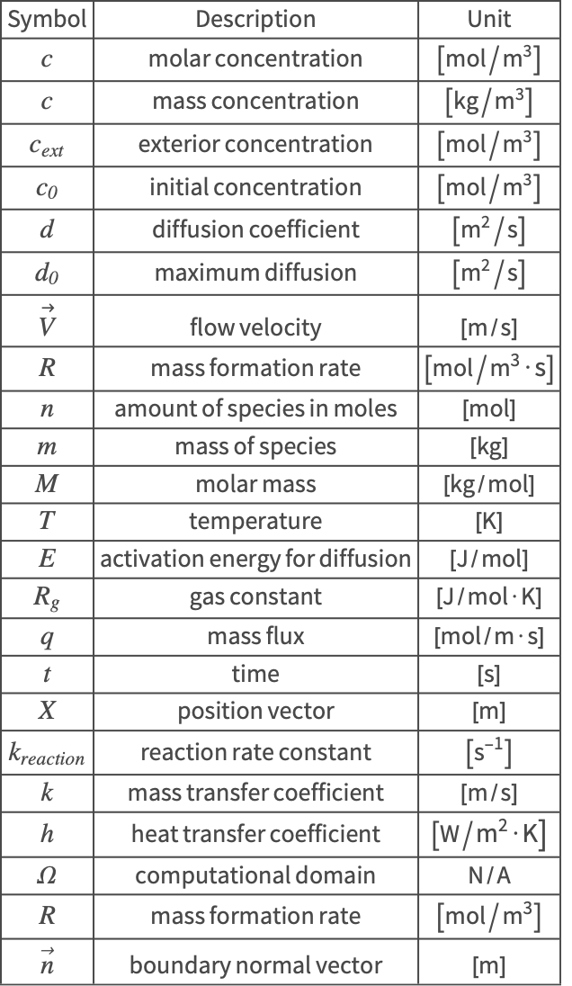
References
1. Fick, A. "Über Diffusion," Annalen der Physik (in German), 94 (1), pp. 59–86 (1855).
2. Wolf, E. E. and Alfani, F. "Catalysts Deactivation by Coking," Catalysis Reviews, vol. 24, pp. 329–371 (1982).
3. Calvo, E. G., Arranz, M. A. and Leton, P. "Effects of Impurities in the Kinetics of Calcite Decomposition," Thermochimica Acta, 170, pp. 7–11 (1990).
4. Fu, J. C., Hagemeir, C. and Moyer, D. L. "A Unified Mathematical Model for Diffusion from Drug Polymer Composite Tablets," Journal of Biomedical Materials Research, vol. 10, no. 5, pp. 743–758 (1976).
5. Parra-Guevara, D. and Skiba, Y. N. "Elements of the Mathematical Modeling in the Control of Pollutants Emissions," Ecological Modelling, vol. 167, no. 3, pp. 263–275 (2003).
6. Goldstein, R.J. and Cho, H. H. "A Review of Mass Transfer Measurements Using Naphthalene Sublimation," Experimental Thermal and Fluid Science, vol. 10, no. 4, pp. 416–434 (1995).
7. Cañizares, P., García-Gómez, J., Fernández de Marcos, I., Rodrigo, M. A. and Lobato, J. "Measurement of Mass-Transfer Coefficients by an Electrochemical Technique," Journal of Chemical Education, vol. 83, no. 8 (2006).
8. LeVeque, R. J. Numerical Methods for Conservation Laws, Birkhäuser Basel (1992).
9. Whitman, G. Walter. "The Two Film Theory of Gas Absorption," International Journal of Heat and Mass Transfer, vol. 5, no. 5, pp. 429–433 (1962).
10. Prausnitz, J. M., Lichtenthaler R. N. and de Azevedo, E. G. Molecular Thermodynamics of Fluid Phase Equilibria, 3rd ed., Prentice Hall PTR, New Jersey (1999).