BaringhausHenzeTest
✖
BaringhausHenzeTest
詳細とオプション


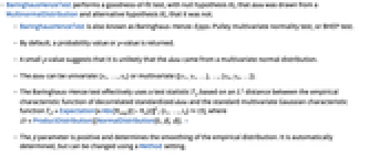
- BaringhausHenzeTestは,data がMultinormalDistributionから取られたという帰無仮説
とそうではないという対立仮説
で適合度検定を実行する.
- BaringhausHenzeTestは,Baringhaus–Henze–Epps–Pulley多変量正規性検定,つまりBHEP検定としても知られている.
- デフォルトで,確率値すなわち
値が返される.
- 小さい
値は data が多変量正規分布から来ている可能性が低いことを示す.
- data は,一変量{x1,…,xn}あるいは多変量{{x1,y1,…},…,{xn,yn,…}}でよい.
- Baringhaus–Henze検定は,事実上,無相関化された標準化 data と標準多変量ガウス特性関数Tβ=Expectation[n Abs[Ψemp[t]-Ψst[t]]2,{t1,…,td}]の間の距離
に基づく経験特性関数検定統計 Tβを使う.ただし,=ProductDistribution[{NormalDistribution[0,β],d}]である. »
- β 母数は正で,経験分布の平滑化を決定する.これは自動的に決定されるが,Method設定で変えることもできる.
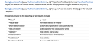
- BaringhausHenzeTest[data,MultinormalDistribution[μ,Σ],"HypothesisTestData"]はHypothesisTestDataオブジェクト htd を返す.これは,htd["property"]として追加的な検定結果および特性の抽出に使うことができる.
- BaringhausHenzeTest[data,MultinormalDistribution[μ,Σ],"property"]を使って直接"property"の値を与えることができる.
- 検定結果のレポートに関連する特性
-
"PValue" 値
"PValueTable" "PValue"のフォーマットされたバージョン "ShortTestConclusion" 検定結果の簡単な説明 "TestConclusion" 検定結果の説明 "TestData" 検定統計と 値
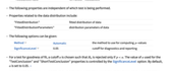
"TestDataTable" "TestData"のフォーマットされたバージョン "TestStatistic" 検定統計 "TestStatisticTable" フォーマットされた"TestStatistic" - 次の特性はどの検定が行われているかに依存しない.
- データ分布に関連する特性
-
"FittedDistribution" データのフィットした分布 "FittedDistributionParameters" データの分布母数 - 使用可能なオプション
-
Method Automatic 値を計算するメソッド
SignificanceLevel 0.05 診断とレポートのための切捨て - 適合度検定では,
のときにのみ
が棄却されるような切捨て
が選択される.特性"TestConclusion"および"ShortTestConclusion"で使われる
の値はSignificanceLevelオプションで制御される.デフォルトで,
は0.05に設定されている. »
- Method->"MonteCarlo"の設定では,入力
と同じ長さのデータ集合が,フィットされた分布を使って
のもとで生成される.次に,BaringhausHenzeTest[si,"TestStatistic"]からのEmpiricalDistributionを使って
値が推定される. »
- Method{method,"SmoothingParameter"β}と設定すると,カスタムの平滑化母数 β を使うことができる.デフォルトは
である.この場合,検定はHenze-Zirkler検定としても知られるものになる. »
例題
すべて開くすべて閉じる例 (3)基本的な使用例

https://wolfram.com/xid/0hu734k865s4h2b7bhbnae-ijo5

https://wolfram.com/xid/0hu734k865s4h2b7bhbnae-hnfx0t

Baringhaus–Henze検定から検定統計を抽出する:

https://wolfram.com/xid/0hu734k865s4h2b7bhbnae-m3chh3

https://wolfram.com/xid/0hu734k865s4h2b7bhbnae-cm7ucc


https://wolfram.com/xid/0hu734k865s4h2b7bhbnae-p7hfx

https://wolfram.com/xid/0hu734k865s4h2b7bhbnae-cr9vsu

スコープ (6)標準的な使用例のスコープの概要
検定 (3)
一変量の正規性についてBaringhaus–Henze検定を行う:

https://wolfram.com/xid/0hu734k865s4h2b7bhbnae-msk3

https://wolfram.com/xid/0hu734k865s4h2b7bhbnae-c8j2us


https://wolfram.com/xid/0hu734k865s4h2b7bhbnae-gsxjf2

多変量の正規性についてBaringhaus–Henze検定を行う:

https://wolfram.com/xid/0hu734k865s4h2b7bhbnae-lqxbgq

https://wolfram.com/xid/0hu734k865s4h2b7bhbnae-mks25


https://wolfram.com/xid/0hu734k865s4h2b7bhbnae-kjd2s

関連特性の抽出のためにHypothesisTestDataオブジェクトを作る:

https://wolfram.com/xid/0hu734k865s4h2b7bhbnae-gtjwh4

https://wolfram.com/xid/0hu734k865s4h2b7bhbnae-licd2


https://wolfram.com/xid/0hu734k865s4h2b7bhbnae-e40fsc

レポート (3)

https://wolfram.com/xid/0hu734k865s4h2b7bhbnae-cqxopz

https://wolfram.com/xid/0hu734k865s4h2b7bhbnae-be6kk1

https://wolfram.com/xid/0hu734k865s4h2b7bhbnae-ef4et7


https://wolfram.com/xid/0hu734k865s4h2b7bhbnae-bfqugt


https://wolfram.com/xid/0hu734k865s4h2b7bhbnae-oi9r56

カスタマイズされたレポート用にBaringhaus–Henze検定の表から項目を取り出す:

https://wolfram.com/xid/0hu734k865s4h2b7bhbnae-s3qsd

https://wolfram.com/xid/0hu734k865s4h2b7bhbnae-ga3bij


https://wolfram.com/xid/0hu734k865s4h2b7bhbnae-gg2n22


https://wolfram.com/xid/0hu734k865s4h2b7bhbnae-65k71

"ShortTestConclusion"と"TestConclusion"を使って検定の結論をレポートする:

https://wolfram.com/xid/0hu734k865s4h2b7bhbnae-bkir6y

https://wolfram.com/xid/0hu734k865s4h2b7bhbnae-cd96sm

https://wolfram.com/xid/0hu734k865s4h2b7bhbnae-ggy9zn


https://wolfram.com/xid/0hu734k865s4h2b7bhbnae-el9mb


https://wolfram.com/xid/0hu734k865s4h2b7bhbnae-c53cri

https://wolfram.com/xid/0hu734k865s4h2b7bhbnae-byyexa


https://wolfram.com/xid/0hu734k865s4h2b7bhbnae-bc67bi

オプション (3)各オプションの一般的な値と機能
Method (2)
Baringhaus–Henze検定に使われる平滑化母数 β を設定する:

https://wolfram.com/xid/0hu734k865s4h2b7bhbnae-kj9pa

https://wolfram.com/xid/0hu734k865s4h2b7bhbnae-qafg

https://wolfram.com/xid/0hu734k865s4h2b7bhbnae-loc4u

モンテカルロ法に基づくメソッドで使われるランダムなシードを設定する:

https://wolfram.com/xid/0hu734k865s4h2b7bhbnae-ccet45

https://wolfram.com/xid/0hu734k865s4h2b7bhbnae-ip8pt1
シードは生成器の状態に影響を与え,結果の 値にもいくらか影響を与える:

https://wolfram.com/xid/0hu734k865s4h2b7bhbnae-pfg0ok

モンテカルロ法と検定母数 β のカスタム設定を使って 値を求める:

https://wolfram.com/xid/0hu734k865s4h2b7bhbnae-h5kxkf


https://wolfram.com/xid/0hu734k865s4h2b7bhbnae-mds8q

SignificanceLevel (1)
"TestConclusion"と"ShortTestConclusion"で使う有意水準を設定する:

https://wolfram.com/xid/0hu734k865s4h2b7bhbnae-bty707

https://wolfram.com/xid/0hu734k865s4h2b7bhbnae-cwgt0i


https://wolfram.com/xid/0hu734k865s4h2b7bhbnae-bf2o0m


https://wolfram.com/xid/0hu734k865s4h2b7bhbnae-sn4sh

アプリケーション (4)この関数で解くことのできる問題の例
Baringhaus–Henze検定の検出力曲線(が偽であるときにこれを拒絶する確率):

https://wolfram.com/xid/0hu734k865s4h2b7bhbnae-dtdyut

https://wolfram.com/xid/0hu734k865s4h2b7bhbnae-bhp5v

https://wolfram.com/xid/0hu734k865s4h2b7bhbnae-fyqopk

https://wolfram.com/xid/0hu734k865s4h2b7bhbnae-eel2vq

基礎となる分布がMultivariateTDistributionであり,検定サイズが0.05,サンプルサイズが43である場合の,Baringhaus–Henze検定の検出力を推定する:

https://wolfram.com/xid/0hu734k865s4h2b7bhbnae-tx1of

連続時間ランダム過程がガウス過程であるかどうかを調べる.非整数ブラウン運動:

https://wolfram.com/xid/0hu734k865s4h2b7bhbnae-cml3p3

https://wolfram.com/xid/0hu734k865s4h2b7bhbnae-e03f59


https://wolfram.com/xid/0hu734k865s4h2b7bhbnae-mjwqkd

https://wolfram.com/xid/0hu734k865s4h2b7bhbnae-k5n1sq

コックス・インガソール・ロス(Cox–Ingersoll–Ross)過程の対数の差:

https://wolfram.com/xid/0hu734k865s4h2b7bhbnae-kuduvz

https://wolfram.com/xid/0hu734k865s4h2b7bhbnae-mr14ho

治療研究の前と後の患者の体重が記録されている.データが多変量正規分布に従っていれば,平均の多変量検定を使って対照群と実験群を識別することができる:

https://wolfram.com/xid/0hu734k865s4h2b7bhbnae-k2w6px

https://wolfram.com/xid/0hu734k865s4h2b7bhbnae-9eqgxb


https://wolfram.com/xid/0hu734k865s4h2b7bhbnae-dwl2bl
BaringhausHenzeTestを使って,データの3群が多変量正規分布に従っているかどうかを判定する:

https://wolfram.com/xid/0hu734k865s4h2b7bhbnae-pheluk


https://wolfram.com/xid/0hu734k865s4h2b7bhbnae-fgd45l


https://wolfram.com/xid/0hu734k865s4h2b7bhbnae-ftpcbx

Baringhaus–Henze検定はContおよびFTの群を棄却しなかった.TTestを使ってこの2群の平均が等しいかどうかを見る:

https://wolfram.com/xid/0hu734k865s4h2b7bhbnae-b6b11r

データが標準非相関二変量正規分布に従っているという仮説を検定する:

https://wolfram.com/xid/0hu734k865s4h2b7bhbnae-cwl6ar

https://wolfram.com/xid/0hu734k865s4h2b7bhbnae-bwdeii

特性と関係 (5)この関数の特性および他の関数との関係
Baringhaus–Henze検定は,データに適用された線形変換が非特異であればアフィン不変である:

https://wolfram.com/xid/0hu734k865s4h2b7bhbnae-cnn3tj

https://wolfram.com/xid/0hu734k865s4h2b7bhbnae-c0toct

https://wolfram.com/xid/0hu734k865s4h2b7bhbnae-bs5yjp

正規性についてのMardiaの結合検定はもまた,同じ特性を有する:

https://wolfram.com/xid/0hu734k865s4h2b7bhbnae-gfijzq

のもとでは,検定統計はLogNormalDistributionに漸近的に従う:

https://wolfram.com/xid/0hu734k865s4h2b7bhbnae-icjpru
検定統計がLogNormalDistribution族からの分布に従うかどうかの検定を行う:

https://wolfram.com/xid/0hu734k865s4h2b7bhbnae-eepa0d


https://wolfram.com/xid/0hu734k865s4h2b7bhbnae-bls0j5


https://wolfram.com/xid/0hu734k865s4h2b7bhbnae-fiq91e

BaringhausHenzeTest統計は,帰無仮説のもとでサンプルの経験特性関数と特性関数の間の距離に基づいている:

https://wolfram.com/xid/0hu734k865s4h2b7bhbnae-kqeayu

https://wolfram.com/xid/0hu734k865s4h2b7bhbnae-i5joq1

https://wolfram.com/xid/0hu734k865s4h2b7bhbnae-dnz20g

https://wolfram.com/xid/0hu734k865s4h2b7bhbnae-w71zl

https://wolfram.com/xid/0hu734k865s4h2b7bhbnae-g9dp2h

BaringhausHenzeTestでレポートされた検定特性の値と比較する:

https://wolfram.com/xid/0hu734k865s4h2b7bhbnae-bx6289

退化したサンプル共分散関数のサンプルについては,検定統計その最大値である4 n を与える:

https://wolfram.com/xid/0hu734k865s4h2b7bhbnae-boe6u

https://wolfram.com/xid/0hu734k865s4h2b7bhbnae-l0h8go


https://wolfram.com/xid/0hu734k865s4h2b7bhbnae-l5ilda

小さい値の平滑化母数 β については,Baringhaus–Henze検定は裾部の動作により敏感である:

https://wolfram.com/xid/0hu734k865s4h2b7bhbnae-j9ss4

https://wolfram.com/xid/0hu734k865s4h2b7bhbnae-trd13

https://wolfram.com/xid/0hu734k865s4h2b7bhbnae-bwhtwi


https://wolfram.com/xid/0hu734k865s4h2b7bhbnae-hb7mj3

おもしろい例題 (1)驚くような使用例や興味深い使用例

https://wolfram.com/xid/0hu734k865s4h2b7bhbnae-lsxpqi

https://wolfram.com/xid/0hu734k865s4h2b7bhbnae-i5e07e


https://wolfram.com/xid/0hu734k865s4h2b7bhbnae-mw4tx7
その成分のヒストグラムをプロットし,標準正規分布の密度関数と比較する:

https://wolfram.com/xid/0hu734k865s4h2b7bhbnae-b1wuas


https://wolfram.com/xid/0hu734k865s4h2b7bhbnae-ri2gt


https://wolfram.com/xid/0hu734k865s4h2b7bhbnae-ffiv0a

Wolfram Research (2015), BaringhausHenzeTest, Wolfram言語関数, https://reference.wolfram.com/language/ref/BaringhausHenzeTest.html.
テキスト
Wolfram Research (2015), BaringhausHenzeTest, Wolfram言語関数, https://reference.wolfram.com/language/ref/BaringhausHenzeTest.html.
CMS
Wolfram Language. 2015. "BaringhausHenzeTest." Wolfram Language & System Documentation Center. Wolfram Research. https://reference.wolfram.com/language/ref/BaringhausHenzeTest.html.
APA
Wolfram Language. (2015). BaringhausHenzeTest. Wolfram Language & System Documentation Center. Retrieved from https://reference.wolfram.com/language/ref/BaringhausHenzeTest.html
BibTeX
@misc{reference.wolfram_2025_baringhaushenzetest, author="Wolfram Research", title="{BaringhausHenzeTest}", year="2015", howpublished="\url{https://reference.wolfram.com/language/ref/BaringhausHenzeTest.html}", note=[Accessed: 30-April-2025
]}
BibLaTeX
@online{reference.wolfram_2025_baringhaushenzetest, organization={Wolfram Research}, title={BaringhausHenzeTest}, year={2015}, url={https://reference.wolfram.com/language/ref/BaringhausHenzeTest.html}, note=[Accessed: 30-April-2025
]}