



BrownForsytheTest
BrownForsytheTest[data]
data の分散が1であるかどうかの検定を行う.
BrownForsytheTest[{data1,data2,…}]
data1, data2, …の分散が等しいかどうかの検定を行う.
BrownForsytheTest[dspec, ]
]
 に対する分散量度の検定を行う.
BrownForsytheTest[dspec, ,"property"]
"property"の値を返す.
詳細とオプション
- BrownForsytheTestは,帰無仮説
 と対立仮説
と対立仮説  で検定を行う.
 -


data 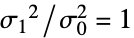
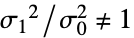
{data1,data2} 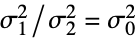
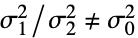
{data1,data2,…} 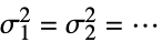
すべてが等しいわけではない - ただし,σi2は dataiの母分散である.
- デフォルトで,確率値すなわち
 値が返される.
  値が小さければ
  が真である可能性は低い.
- dspec 中の data は一変量{x1,x2,…}でなければならない.
- 引数
 は任意の正の実数でよい.特に指定がない限り
 のデフォルト値は1で,dspec 内のグループ数が2より多い場合は無視される.
 - BrownForsytheTestはデータが正規分布に従うと仮定する.
- BrownForsytheTestはLeveneTestに比べ正規性の仮定に対する感受性が低い.
- BrownForsytheTest[data,
 ,"HypothesisTestData"]は htd["property"]の形で追加的な検定結果と特性の抽出に利用できるHypothesisTestDataオブジェクト htd を返す.
 - BrownForsytheTest[data,
 ,"property"]を使って直接"property"の値を与えることができる.
 - 検定結果のレポートに関連する特性
-
"DegreesOfFreedom" 検定に使用する自由度 "PValue"  値のリスト
値のリスト"PValueTable"  値のフォーマットされた表
"ShortTestConclusion" 検定結果の簡単な説明 "TestConclusion" 検定結果の説明 "TestData" 検定統計と  値のペアのリスト
"TestDataTable"  値と検定統計のフォーマットされた表
"TestStatistic" 検定統計のリスト "TestStatisticTable" 検定統計のフォーマットされた表 - サイズ
 のサンプル1つが与えられた場合,BrownForsytheTestはFisherRatioTestに等しい.
 - サンプルが
 個の場合,BrownForsytheTestはAbs[dataij-Mean[dataij]]のMeanを関数 fn で置き換えるLeveneTestを修正したものになる.関数 fn には一般にMedianが選ばれるが,データの裾部が重い場合にはTrimmedMean[#,1/10]&が使われる.
 - 使用可能なオプション
-
AlternativeHypothesis "Unequal" 対立仮説のための不等式 SignificanceLevel 0.05 診断とレポートのための切捨て VerifyTestAssumptions Automatic どの診断検定を実行するかを設定する - BrownForsytheTestでは,
 のときにのみ
  が棄却されるような切捨て
  が選ばれる."TestConclusion"および"ShortTestConclusion"特性に使われる
  の値はSignificanceLevelオプションで制御される.値
  は正規性と対称性の検定を含む仮定の診断検定にも使われる.デフォルトで
  は0.05に設定される.
 - BrownForsytheTestのVerifyTestAssumptionsの名前付き設定
-
"Normality" すべてのデータが正規分布に従うことを検証する
例題
すべて開く すべて閉じる例 (2)
data = RandomVariate[NormalDistribution[], {2, 100}];BrownForsytheTest[data]さらに特性を抽出するためにHypothesisTestDataオブジェクトを作る:
ℋ = BrownForsytheTest[data, Automatic, "HypothesisTestData"]ℋ["Properties"]SeedRandom["test"];
data1 = RandomVariate[NormalDistribution[0, 1], 100];
data2 = RandomVariate[NormalDistribution[0, 2.5], 250];BrownForsytheTest[{data1, data2}, 1 / 4, "TestDataTable"]Variance[data1] / Variance[data2]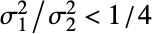
BrownForsytheTest[{data1, data2}, 1 / 4, AlternativeHypothesis -> "Less"]スコープ (10)
検定 (8)
SeedRandom[1];
data1 = RandomVariate[NormalDistribution[], 500];
data2 = RandomVariate[NormalDistribution[1, .3], 500];

BrownForsytheTest[data1]

BrownForsytheTest[data2]SeedRandom["val"];data1 = RandomVariate[NormalDistribution[0, 2], 10^4];
data2 = RandomVariate[NormalDistribution[0, 2.1], 10^4];BrownForsytheTest[data1, 2^2]BrownForsytheTest[data2, 2^2]SeedRandom["2"];data1 = RandomVariate[NormalDistribution[0, 3], 500];
data2 = RandomVariate[NormalDistribution[1, 3], 500];

BrownForsytheTest[{data1, data2}]Brown–Forsythe検定の  値のサンプルのヒストグラム:
sample = Table[Quiet@BrownForsytheTest[{RandomVariate[NormalDistribution[0, 3], 100], RandomVariate[NormalDistribution[1, 3], 100]}], {5 10 ^ 3}];Histogram[sample, Automatic, PDF]
data3 = RandomVariate[NormalDistribution[10, 1], 350];BrownForsytheTest[{data1, data3}]SeedRandom["ratio"];data1 = RandomVariate[NormalDistribution[0, 2], 500];
data2 = RandomVariate[NormalDistribution[0, 1], 500];Subscript[σ, 0] = 4;BrownForsytheTest[{data1, data2}, Subscript[σ, 0]]BrownForsytheTest[{data2, data1}, 1 / Subscript[σ, 0]]
BrownForsytheTest[{data2, data1}, Subscript[σ, 0]]SeedRandom["3"];data1 = RandomVariate[NormalDistribution[10, 1], 500];
data2 = RandomVariate[NormalDistribution[0, 1], 200];
data3 = RandomVariate[NormalDistribution[-3, 1], 400];BrownForsytheTest[{data1, data2, data3}]繰り返し特性を抽出するためにHypothesisTestDataオブジェクトを作成する:
SeedRandom["prop"];data = RandomVariate[NormalDistribution[], {2, 10^4}];ℋ = BrownForsytheTest[data, 1, "HypothesisTestData"];ℋ["Properties"]HypothesisTestDataオブジェクトから特性をいくつか抽出する:
SeedRandom["obj"];data = RandomVariate[NormalDistribution[], {2, 10^4}];ℋ = BrownForsytheTest[data, 1, "HypothesisTestData"];
ℋ["PValue"]ℋ["TestStatistic"]ℋ["DegreesOfFreedom"]SeedRandom["m"];data = RandomVariate[NormalDistribution[], {2, 100}];ℋ = BrownForsytheTest[data, 1, "HypothesisTestData"];
ℋ["PValue", "TestStatistic", "DegreesOfFreedom"]レポート (2)
SeedRandom["tab"];data = RandomVariate[NormalDistribution[], {2, 10^3}];ℋ = BrownForsytheTest[data, 1, "HypothesisTestData"];ℋ["TestDataTable"]ℋ["TestData"]
SeedRandom["tab"];data = RandomVariate[NormalDistribution[], {3, 10^4}];ℋ = BrownForsytheTest[data, 1, "HypothesisTestData"];ℋ["PValueTable"]
ℋ["PValue"]ℋ["TestStatisticTable"]ℋ["TestStatistic"]オプション (8)
AlternativeHypothesis (3)
SeedRandom["alt"];data = RandomVariate[NormalDistribution[], 100];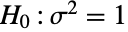
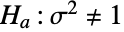
BrownForsytheTest[data, 1, AlternativeHypothesis -> "Unequal"]BrownForsytheTest[data, 1, AlternativeHypothesis -> Automatic]SeedRandom["alt"];data = RandomVariate[NormalDistribution[0, 1.25], 100];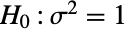
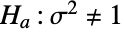
BrownForsytheTest[data, Automatic, AlternativeHypothesis -> "Unequal"]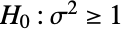
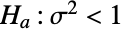
BrownForsytheTest[data, Automatic, AlternativeHypothesis -> "Less"]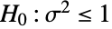
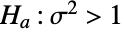
BrownForsytheTest[data, Automatic, AlternativeHypothesis -> "Greater"]SeedRandom["null"];
data1 = RandomVariate[NormalDistribution[0, .9], 100];
data2 = RandomVariate[NormalDistribution[0, 1], 100];Variance[data1] / Variance[data2]

BrownForsytheTest[{data1, data2}, 1, AlternativeHypothesis -> "Less"]

BrownForsytheTest[{data1, data2}, 1.5, AlternativeHypothesis -> "Less"]SignificanceLevel (2)
data = BlockRandom[SeedRandom[5];RandomVariate[StudentTDistribution[3], 50]];BrownForsytheTest[data, 1, SignificanceLevel -> .005]BrownForsytheTest[data, 1, SignificanceLevel -> Automatic]
有意水準は"TestConclusion"と"ShortTestConclusion"にも使われる:
data = BlockRandom[SeedRandom[1];RandomVariate[NormalDistribution[0, 1], 100]];ℋ1 = BrownForsytheTest[data, 1.5, "HypothesisTestData", SignificanceLevel -> .05];ℋ2 = BrownForsytheTest[data, 1.5, "HypothesisTestData", SignificanceLevel -> .01];ℋ1["TestConclusion"]//TraditionalFormℋ2["TestConclusion"]//TraditionalFormℋ1["ShortTestConclusion"]ℋ2["ShortTestConclusion"]VerifyTestAssumptions (3)
診断は,AllあるいはNoneを使ってまとめて制御することができる:
SeedRandom["ver"];data1 = RandomVariate[StudentTDistribution[3], 1000];
data2 = RandomVariate[NormalDistribution[0, Sqrt[3]], 1000];BrownForsytheTest[{data1, data2}, 1 / 4, VerifyTestAssumptions -> All]
BrownForsytheTest[{data1, data2}, 1 / 4, VerifyTestAssumptions -> None]SeedRandom["ver"];data1 = RandomVariate[StudentTDistribution[2], 1000];
data2 = RandomVariate[NormalDistribution[0, Sqrt[3]], 1000];BrownForsytheTest[{data1, data2}, 1 / 4, VerifyTestAssumptions -> "Normality"]
仮定値をTrueに設定する:
BrownForsytheTest[{data1, data2}, 1 / 4, VerifyTestAssumptions -> "Normality" -> True]シミュレーションを行う場合は,診断検定を行わないようにすると有益であることが多い:
SeedRandom["test"];data = RandomVariate[NormalDistribution[], {1000, 100}];AbsoluteTiming[T = Quiet@BrownForsytheTest[#, Automatic, "TestStatistic"]& /@ data;]検定の仮定は意図的に有効になっているので,時間が大幅に短縮できる:
AbsoluteTiming[T2 = Quiet@BrownForsytheTest[#, Automatic, "TestStatistic", VerifyTestAssumptions -> None]& /@ data;]SmoothHistogram[{T, T2}]アプリケーション (1)
Brown–Forsythe検定を使って,等しい平均の  検定におよその自由度が必要であるかどうかを判断する:
data1 = {-0.509, 2.25, -0.553, 1.234, 0.527, 0.319, 1.315, 1.024, 0.212, 0.835, 0.215, 0.652, 0.705, 0.683, -0.804};data2 = {-0.714, 4.559, 1.546, 2.819, -0.814, -4.146, 0.409, -3.241, -3.987, -2.739, 0.254, -4.887, -7.827, 0.424, -0.095};L[x_] := Length[x];v[x_] := Variance[x]
ttest[𝒹1_, 𝒹2_, μ0_, df_] := With[{t = (Mean[𝒹1] - Mean[𝒹2] - μ0/Sqrt[(v[𝒹1]/L[𝒹1]) + (v[𝒹2]/L[𝒹2])])}, {"T" -> t, "p" -> 2 Min[SurvivalFunction[StudentTDistribution[df], t], CDF[StudentTDistribution[df], t]], "df" -> df}]2つのサンプルが等しい分散を持つ場合には,以下の自由度を使用することができる.その他の場合は,Satterthwaite近似が必要である:
evDF[𝒹1_, 𝒹2_] := L[𝒹1] + L[𝒹2] - 2SatterthwaiteDF[𝒹1_, 𝒹2_] := (((v[𝒹1]/L[𝒹1]) + (v[𝒹2]/L[𝒹2]))^2/((v[𝒹1]/L[𝒹1]))^2 / (L[𝒹1] - 1) + ((v[𝒹2]/L[𝒹2]))^2 / (L[𝒹2] - 1))Brown–Forsythe検定は,分散が等しくないことを示唆する:
BrownForsytheTest[{data1, data2}, 1, "TestDataTable"]0.05レベルでは,自由度の選択が検定の結論に影響を与える:
ttest[data1, data2, 0, evDF[data1, data2]]ttest[data1, data2, 0, SatterthwaiteDF[data1, data2]]TTestは,Satterthwaite近似を自動的に使うことを決定する:
TTest[{data1, data2}, 0, {"TestDataTable", "DegreesOfFreedom"}]特性と関係 (8)
1つのデータ集合が与えられた場合,Brown–Forsythe検定はFisherRatioTestに等しい:
SeedRandom["e"];data = RandomVariate[NormalDistribution[], 100];BrownForsytheTest[data]FisherRatioTest[data]長さ  の1つのデータ集合が与えられた場合,検定統計は
  においてChiSquareDistribution[n-1]に従う:
SeedRandom["chi"];data = RandomVariate[NormalDistribution[], {1000, 100}];T = BrownForsytheTest[#, Automatic, "TestStatistic", VerifyTestAssumptions -> None]& /@ data;Show[SmoothHistogram[T], Plot[PDF[ChiSquareDistribution[99], x], {x, 50, 160}, PlotStyle -> Orange]]
EstimatedDistribution[T, ChiSquareDistribution[df]]DistributionFitTest[T, ChiSquareDistribution[99]]長さが 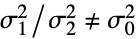 と
と 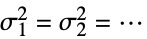 である2つのデータ集合が与えられた場合,検定統計は
  においてFRatioDistribution[1,n+m-2]に従う:
n = 100;
m = 75;
SeedRandom["F"];
data1 = RandomVariate[NormalDistribution[], {1000, n}];
data2 = RandomVariate[NormalDistribution[], {1000, m}];T = MapThread[BrownForsytheTest[{#1, #2}, Automatic, "TestStatistic", VerifyTestAssumptions -> None]&, {data1, data2}];Show[Histogram[T, {0.2}, "PDF"], Plot[PDF[FRatioDistribution[1, n + m - 2], x], {x, 0, 8}, PlotRange -> {0, 1}]]DistributionFitTest[T, FRatioDistribution[1, n + m - 2], "TestConclusion"]Brown–Forsythe検定は,2つのデータ集合を与えられたFisherRatioTestに比べて,正規性の仮定を感知する度合が低い:
SeedRandom["F"];data1 = RandomVariate[LaplaceDistribution[1, 2], {1000, 100}];
data2 = RandomVariate[LaplaceDistribution[1, 2], {1000, 75}];fisher = MapThread[FisherRatioTest[{#1, #2}, VerifyTestAssumptions -> None]&, {data1, data2}];levene = MapThread[BrownForsytheTest[{#1, #2}, VerifyTestAssumptions -> None]&, {data1, data2}];Fisher比率検定は, 値を過小評価しがちで,タイプIエラーをより多く犯す:
Histogram[{fisher, levene}, Automatic, "PDF"]Subscript[n, 1] = 100;Subscript[n, 2] = 75;Subscript[σ, 0] = 2;SeedRandom["2"];data1 = RandomVariate[NormalDistribution[0, Subscript[σ, 0]], Subscript[n, 1]];
data2 = RandomVariate[NormalDistribution[0, 1], Subscript[n, 2]];Subscript[n, t] = Subscript[n, 1] + Subscript[n, 2];bfor[d1_, d2_, f_] := Block[{μZ1, μZ2, z1, z2, μZZ},
z1 = Abs@Standardize[d1, f, 1&];
z2 = Subscript[σ, 0]Abs@Standardize[d2, f, 1&];
μZ1 = Mean[z1];μZ2 = Mean[z2];
μZZ = (Subscript[n, 1] μZ1 + Subscript[n, 2] μZ2/Subscript[n, t]);
(Subscript[n, t] - 2)(Subscript[n, 1](μZ1 - μZZ)^2 + Subscript[n, 2](μZ2 - μZZ)^2/(z1 - μZ1).(z1 - μZ1) + (z2 - μZ2).(z2 - μZ2))]通常,Medianが標準化関数として使われる:
bfor[data1, data2, Median]BrownForsytheTest[{data1, data2}, Subscript[σ, 0] ^ 2, "TestStatistic"]裾部が重いデータには,10%のTrimmedMeanが使われる:
data3 = RandomVariate[CauchyDistribution[0, Subscript[σ, 0]], Subscript[n, 1]];
data4 = RandomVariate[CauchyDistribution[0, 1], Subscript[n, 2]];bfor[data3, data4, TrimmedMean[#, .1]&]BrownForsytheTest[{data3, data4}, Subscript[σ, 0] ^ 2, "TestStatistic", VerifyTestAssumptions -> None]LeveneTestは等しいが,必ずMeanを標準化に使用する:
bfor[data1, data2, Mean]LeveneTest[{data1, data2}, Subscript[σ, 0] ^ 2, "TestStatistic"]Subscript[n, 1] = 1000;Subscript[n, 2] = 750;Subscript[n, 3] = 1500;SeedRandom["3"];data1 = RandomVariate[NormalDistribution[-4, 3], Subscript[n, 1]];
data2 = RandomVariate[NormalDistribution[1, 3], Subscript[n, 2]];
data3 = RandomVariate[NormalDistribution[5, 3], Subscript[n, 3]];Subscript[n, t] = Subscript[n, 1] + Subscript[n, 2] + Subscript[n, 3];bfor3[d1_, d2_, d3_] := Block[{μZ1, μZ2, μZ3, z1, z2, z3, μZZ},
z1 = Abs[d1 - Median[d1]];
z2 = Abs[d2 - Median[d2]];
z3 = Abs[d3 - Median[d3]];
μZ1 = Mean[z1];μZ2 = Mean[z2];μZ3 = Mean[z3];
μZZ = (Subscript[n, 1]μZ1 + Subscript[n, 2]μZ2 + Subscript[n, 3]μZ3/Subscript[n, t]);
((Subscript[n, t] - 3)/2)(Subscript[n, 1](μZ1 - μZZ)^2 + Subscript[n, 2](μZ2 - μZZ)^2 + Subscript[n, 3](μZ3 - μZZ)^2/Total[(z1 - μZ1) ^ 2] + Total[(z2 - μZ2) ^ 2] + Total[(z3 - μZ3) ^ 2])]bfor3[data1, data2, data3]BrownForsytheTest[{data1, data2, data3}, 1, "TestStatistic"]Brown–Forsythe検定は,入力がTimeSeriesのときにだけ値に使うことができる:
ts = TemporalData[TimeSeries, {{{1.224578634529677, 0.47929635789978015, 0.6572781300178168,
    0.21496048742669355, 0.7299608014554928, -0.2495111111278263, -1.3286551762002712,
    0.552725018274874, 0.19272112205837066, 1.1809144012420882, -1.1671 ... 40938613662046, 1.052394590214582, 0.9345044123980388, 0.38537803109557855,
    -0.48660931166089394, -0.71203560340161}}, {{0, 100, 1}}, 1, {"Continuous", 1},
{"Discrete", 1}, 1, {ValueDimensions -> 1, ResamplingMethod -> None}}, False, 10.1];BrownForsytheTest[ts]BrownForsytheTest[ts["Values"]]Brown–Forsythe検定は,入力がTemporalDataのときには,あらゆる値に使うことができる:
td = TemporalData[Automatic, {{{-0.25275046867718637, -0.7175779198306353, -1.9370139837317764,
    0.006665621735740701, -0.3730807122324292, 0.6740106823161018, 0.8562214990564344,
    0.955785083955732, 1.7020898014886303, 1.8523009430646802, 0.244 ... 3951759101545, -1.1611722313627828, 1.1602446901533021,
    1.1052173095128992, 1.1089143920161917, -0.13837156328402}}, {{0, 100, 1}}, 2,
  {"Continuous", 2}, {"Discrete", 1}, 1, {ValueDimensions -> 1, ResamplingMethod -> None}}, False,
10.1];BrownForsytheTest[td]data = td["ValueList"]//Flatten;
BrownForsytheTest[data]{data1, data2} = td["ValueList"];BrownForsytheTest[{data1, data2}]考えられる問題 (3)
Brown–Forsythe検定は,データがNormalDistributionから取られたと仮定する:
SeedRandom["n"];data = RandomVariate[LaplaceDistribution[1, 2], {2, 100}];BrownForsytheTest[data, 1, "TestDataTable"]
非正規データにはConoverTestかSiegelTukeyTestを使う:
ConoverTest[data, 1, "TestDataTable"]SiegelTukeyTest[data, 1, "TestDataTable"]グループが2より多いとき,Brown–Forsythe検定は引数  を無視する:
SeedRandom["1"];data = RandomVariate[NormalDistribution[1, 2], {4, 100}];Length[data]BrownForsytheTest[data, 2, "TestDataTable"]
データ中に2より多くのグループがあるとき,Brown–Forsy統計は対立仮説に両側検定しか認めない:
SeedRandom["alt"];data = RandomVariate[NormalDistribution[1, 2], {4, 100}];BrownForsytheTest[data, 1, AlternativeHypothesis -> "Unequal"]BrownForsytheTest[data, 1, AlternativeHypothesis -> "Greater"]
BrownForsytheTest[data, 1, AlternativeHypothesis -> "Less"]
おもしろい例題 (1)

SeedRandom["neat"];data = RandomVariate[NormalDistribution[], {250, 100}];T1 = BrownForsytheTest[#, 1, "TestStatistic", VerifyTestAssumptions -> None]& /@ data;T2 = BrownForsytheTest[#, 3, "TestStatistic", VerifyTestAssumptions -> None]& /@ data;SmoothHistogram[{T1, T2}, Filling -> Axis, PlotLegends -> {"SubscriptBox[H, 0] is True", "SubscriptBox[H, 0] is False"}, PlotStyle -> Thick]テキスト
Wolfram Research (2010), BrownForsytheTest, Wolfram言語関数, https://reference.wolfram.com/language/ref/BrownForsytheTest.html (2017年に更新).
CMS
Wolfram Language. 2010. "BrownForsytheTest." Wolfram Language & System Documentation Center. Wolfram Research. Last Modified 2017. https://reference.wolfram.com/language/ref/BrownForsytheTest.html.
APA
Wolfram Language. (2010). BrownForsytheTest. Wolfram Language & System Documentation Center. Retrieved from https://reference.wolfram.com/language/ref/BrownForsytheTest.html