CompleteIntegral

CompleteIntegral
CompleteIntegral[pde,u,{x1,…,xn}]
给出一阶偏微分方程 pde 的全积分 u,其中自变量为 {x1,…,xn}.
更多信息和选项
- 具有 n 个变量的一阶偏微分方程 (PDE) 的全积分是依赖于 n 个独立任意常数 c1,c2,…,cn 的解.
- 全积分通常用于生成 PDE 的完整解集.
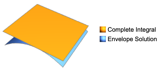
- 满足特定初始条件的 PDE 的解可以通过构建依赖于
 个参数的简单解的平滑变化子族的包络来获得,如图所示. »
 - The output from CompleteIntegral 的输出由依赖函数 u 或 u[x1,…,xn] 控制,如在 DSolve 中一样.
- CompleteIntegral 可以根据 Solve 给出隐式解.
- CompleteIntegral 可以给出包含无法明确执行的 Inactive 和与积分的解. 在这种情况下使用变量 K[1], K[2], ….
- 可以指定偏微分方程的边界条件以获得全积分中不受任意常数影响的偏微分方程的特解. »
- 可以提供以下选项:
-
Assumptions $Assumptions 参数假设 GeneratedParameters C 如何命名生成的参数 Method Automatic 使用什么方法 - GeneratedParameters 控制生成参数的形式; 这些默认是常数 C[n].
范例
打开所有单元 关闭所有单元基本范例 (3)
CompleteIntegral[D[u[x, y], x] - D[u[x, y], y] ^ 2 == Cos[x] , u[x, y], {x, y}]Plot3D[u[x, y] /. %[[1]] /. {C[1] -> 1 / 3, C[2] -> 1}, {x, 0, 10Pi}, {y, 0, 5}]CompleteIntegral[D[w[x, y], x] - y w[x, y]D[w[x, y], y] == w[x, y] + x ^ 2 - 1, w, {x, y}]Simplify[D[w[x, y], x] - y w[x, y]D[w[x, y], y] == w[x, y] + x ^ 2 - 1 /. %]CompleteIntegral[D[u[x, y, z], x] ^ 3 == D[u[x, y, z], y] + D[u[x, y, z], z], u[x, y, z], {x, y, z}]CompleteIntegral[D[u[x, y, z], x] ^ 3 == D[u[x, y, z], y] + D[u[x, y, z], z] && u[0, 1, 1] == 1 && u[1, 0, 1] == 1 && u[0, 0, 1] == 1 / 2, u[x, y, z], {x, y, z}]范围 (5)
CompleteIntegral[D[u[x, y], x] + D[u[x, y], y] == u[x, y] ^ 2, u[x, y], {x, y}]CompleteIntegral[D[u[x, y], x] + D[u[x, y], y] == u[x, y] ^ 2, u, {x, y}]Simplify[D[u[x, y], x] + D[u[x, y], y] /. %]CompleteIntegral[D[w[x, y], x] - 1 / Sin[y]w[x, y]D[w[x, y], y] == 1 / x w[x, y] + Log[x], w[x, y], {x, y}]CompleteIntegral[D[w[x, y], x] - y w[x, y]D[w[x, y], y] == x w[x, y] + x ^ 2 - 1, w[x, y], {x, y}]CompleteIntegral[ D[u[x, y], x] - x D[u[x, y], y] == 0, u[x, y], {x, y}]与 DSolve 给出的解比较:
DSolve[ D[u[x, y], x] - x D[u[x, y], y] == 0, u[x, y], {x, y}]CompleteIntegral[ D[u[x, y], x] - u[x, y] D[u[x, y], y] == 0, u[x, y], {x, y}]与 DSolve 给出的解比较:
DSolve[ D[u[x, y], x] - u[x, y] D[u[x, y], y] == 0, u[x, y], {x, y}]应用 (2)
ClairautEquation = u[x, y] == x * D[u[x, y], {x}] + y * D[u[x, y], {y}] +
(1 / 2) * (D[u[x, y], {x}] ^ 2 + D[u[x, y], {y}] ^ 2);csol = u[x, y] /. CompleteIntegral[ClairautEquation, u, {x, y}][[1]]psol = csol /. {C[2] -> -1}Solve[(D[psol, C[1]]) == 0, C[1]]envelope = psol /. %[[1]]//TogetherClairautEquation /. {u -> Function[{x, y}, Evaluate[envelope]]}//SimplifyAnimate[...]HamiltonJacobiEqn = D[u[t, x], t] + D[u[t, x], x] ^ 2 == 0;ci = CompleteIntegral[HamiltonJacobiEqn, u[t, x], {t, x}]sol = u[t, x] /. ci[[1]] /. {C[1] -> 0, C[2] -> a}Solve[D[sol, a] == 0, a]envelopsol = sol /. %[[1]]Plot3D[Evaluate[envelopsol], {t, -4, 4}, {x, -3, 3}, PlotRange -> All]HamiltonJacobiEqn /. u -> Function[{t, x}, Evaluate[envelopsol]]属性和关系 (2)
CompleteIntegral 求非线性偏微分方程的全积分:
deqn = D[u[x, y], x] + D[u[x, y], y] ^ 2 == 1;CompleteIntegral[deqn, u[x, y], {x, y}]DSolve 返回带有警告消息的相同解:
DSolve[deqn, u[x, y], {x, y}]
使用 CompleteIntegral 求线性偏微分方程的全积分:
deqn = D[u[x, y], x] + D[u[x, y], y] == 1;CompleteIntegral[deqn, u[x, y], {x, y}]DSolve 返回此偏微分方程的通解:
DSolve[deqn, u[x, y], {x, y}]
Wolfram Research (2021),CompleteIntegral,Wolfram 语言函数,https://reference.wolfram.com/language/ref/CompleteIntegral.html.
文本
Wolfram Research (2021),CompleteIntegral,Wolfram 语言函数,https://reference.wolfram.com/language/ref/CompleteIntegral.html.
CMS
Wolfram 语言. 2021. "CompleteIntegral." Wolfram 语言与系统参考资料中心. Wolfram Research. https://reference.wolfram.com/language/ref/CompleteIntegral.html.
APA
Wolfram 语言. (2021). CompleteIntegral. Wolfram 语言与系统参考资料中心. 追溯自 https://reference.wolfram.com/language/ref/CompleteIntegral.html 年