

ElectricPotentialCondition
ElectricPotentialCondition[pred,vars,pars]
represents an electric potential surface boundary condition for PDEs with predicate pred indicating where it applies, with model variables vars and global parameters pars.
ElectricPotentialCondition[pred,vars,pars,lkey]
represents an electric potential surface boundary condition with local parameters specified in pars[lkey].
Details
- ElectricPotentialCondition specifies a Dirichlet boundary condition for ElectrostaticPDEComponent and ElectricCurrentPDEComponent.
- ElectricPotentialCondition specifies a boundary condition for ElectrostaticPDEComponent and ElectricCurrentPDEComponent.
- ElectricPotentialCondition is typically used to set a specific electric potential on the boundary. Common examples include capacitive devices charged by applying a voltage difference.
- ElectricPotentialCondition sets a specific electric potential on the boundary with dependent variable
 and independent variables
  .
. - Stationary variables vars are vars={V[x1,…,xn],{x1,…,xn}}.
- Frequency-dependent variables vars are vars={V[x1,…,xn],ω,{x1,…,xn}}.
- The stationary or frequency domain electric potential condition ElectricPotentialCondition model
 where
where  [
[![TemplateBox[{InterpretationBox[, 1], "V", volts, "Volts"}, QuantityTF]](Files/ElectricPotentialCondition.en/6.png "TemplateBox[{InterpretationBox[, 1], \"V\", volts, \"Volts\"}, QuantityTF]") ] is a given surface potential.
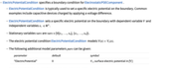
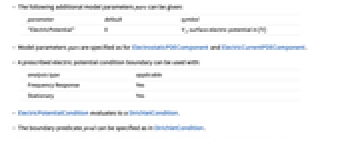
] is a given surface potential. - The following additional model parameters pars can be given:
-
parameter default symbol "ElectricPotential" - 0
 , surface electric potential in [
![TemplateBox[{InterpretationBox[, 1], "V", volts, "Volts"}, QuantityTF]](Files/ElectricPotentialCondition.en/8.png "TemplateBox[{InterpretationBox[, 1], \"V\", volts, \"Volts\"}, QuantityTF]") ]
] - Model parameters pars are specified as for ElectrostaticPDEComponent and ElectricCurrentPDEComponent.
- A prescribed electric potential condition boundary can be used with:
-
analysis type applicable Frequency Response Yes Stationary Yes - ElectricPotentialCondition evaluates to a DirichletCondition.
- The boundary predicate pred can be specified as in DirichletCondition.
- If the ElectricPotentialCondition depends on parameters
 that are specified in the association pars as …,keypi…,pivi,…, the parameters
  are replaced with
  .
.
Examples
open all close allBasic Examples (3)
Set up an electric potential surface boundary condition:
Set up a default electric potential surface boundary condition:
Compute the electric potential distribution with model variables ![]() and parameters
and parameters ![]() with an electric potential
with an electric potential ![]() of
of ![]() [
[![]() ] at the left boundary and a ground potential at the right boundary.
] at the left boundary and a ground potential at the right boundary.
Specify model variables and electrostatic parameters:
Scope (4)
Define model variables vars for an electrostatic analysis with model parameters pars and multiple specific parameter boundary conditions:
1D (1)
Compute the electric potential distribution between two parallel plates separated by a distance ![]() [
[![]() ] and positioned normal to the
] and positioned normal to the ![]() axis. The left plate is maintained at a constant potential
axis. The left plate is maintained at a constant potential ![]() [
[![]() ], whereas the right plate is grounded,
], whereas the right plate is grounded, ![]() . The region between the plates is characterized by a relative permittivity
. The region between the plates is characterized by a relative permittivity ![]() and a uniform electron charge density
and a uniform electron charge density ![]() [
[![]() ]. The equation to use in the model is given by:
]. The equation to use in the model is given by:
Set up the electrostatic model variables ![]() :
:
Specify electrostatic model parameters:
2D (1)
Solve for the electric scalar potential in a three-bar electric switch with an electrical conductivity of ![]() . The equation to use in the model is given by:
. The equation to use in the model is given by:
Set up the electrostatic model variables ![]() :
:
Specify an electrical conductivity ![]() :
:
Specify ground potential at the lower boundary:
Specify an electric potential of ![]() [
[![]() ] at the upper boundary:
] at the upper boundary:
3D (1)
Model a simplified bushing insulator of a transformer with an electric potential condition at the inner walls, which are in contact with the high-voltage conductor, and a ground potential boundary at one of the surface plates (![]() ). The equation to use in the model is given by:
). The equation to use in the model is given by:
Set up the electrostatic model variables ![]() :
:
Specify a relative permittivity ![]() :
:
Specify a ground potential at the surface ![]() :
:
Text
Wolfram Research (2024), ElectricPotentialCondition, Wolfram Language function, https://reference.wolfram.com/language/ref/ElectricPotentialCondition.html (updated 2024).
CMS
Wolfram Language. 2024. "ElectricPotentialCondition." Wolfram Language & System Documentation Center. Wolfram Research. Last Modified 2024. https://reference.wolfram.com/language/ref/ElectricPotentialCondition.html.
APA
Wolfram Language. (2024). ElectricPotentialCondition. Wolfram Language & System Documentation Center. Retrieved from https://reference.wolfram.com/language/ref/ElectricPotentialCondition.html