

GreenFunction
GreenFunction[{ℒ[u[x]],ℬ[u[x]]},u,{x,xmin,xmax},y]
gives a Green's function for the linear differential operator ℒ with boundary conditions ℬ in the range xmin to xmax.
GreenFunction[{ℒ[u[x1,x2,…]],ℬ[u[x1,x2,…]]},u,{x1,x2,…}∈Ω,{y1,y2,…}]
gives a Green's function for the linear partial differential operator ℒ over the region Ω.
GreenFunction[{ℒ[u[x,t]],ℬ[u[x,t]]},u,{x,xmin,xmax},t,{y,τ}]
gives a Green's function for the linear time-dependent operator ℒ in the range xmin to xmax.
GreenFunction[{ℒ[u[x1,…,t]],ℬ[u[x1,…,t]]},u,{x1,…}∈Ω,t,{y1,…,τ}]
gives a Green's function for the linear time-dependent operator ℒ over the region Ω.
Details and Options
- GreenFunction represents the response of a system to an impulsive DiracDelta driving function.
- GreenFunction for a differential operator
 is defined to be a solution
  of
of ![L(G(x;y))=TemplateBox[{{x, -, y}}, DiracDeltaSeq]](Files/GreenFunction.en/3.png "L(G(x;y))=TemplateBox[{{x, -, y}}, DiracDeltaSeq]") that satisfies the given homogeneous boundary conditions
that satisfies the given homogeneous boundary conditions  .
. - A particular solution of
 with homogeneous boundary conditions
  can be obtained by performing a convolution integral
  .
. - GreenFunction for a time-dependent differential operator
 is defined to be a solution
  of
of ![L(G(x,t;y,tau))=TemplateBox[{{x, -, y}}, DiracDeltaSeq]TemplateBox[{{t, -, tau}}, DiracDeltaSeq]](Files/GreenFunction.en/10.png "L(G(x,t;y,tau))=TemplateBox[{{x, -, y}}, DiracDeltaSeq]TemplateBox[{{t, -, tau}}, DiracDeltaSeq]") that satisfies the given homogeneous boundary conditions
that satisfies the given homogeneous boundary conditions  .
. - A particular solution of
 with homogeneous boundary conditions
  can be obtained by performing a convolution integral
  .
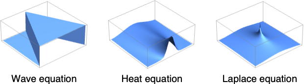
. - The Green's functions for classical PDEs have characteristic geometrical properties:
 is given as an expression in
  and
and  if the dependent variable is of the form
  , and as a pure function with formal parameters
  and
and  if the dependent variable is of the form
  instead of
  . »
. »- The region Ω can be anything for which RegionQ[Ω] is True.
- All the necessary initial and boundary conditions for ODEs must be specified in
 .
. - Boundary conditions for PDEs must be specified using DirichletCondition or NeumannValue in
 .
. - Assumptions on parameters may be specified using the Assumptions option.
Examples
open all close allBasic Examples (2)
Green's function for a boundary value problem:
GreenFunction[{-u''[x], u[0] == 0, u[1] == 0}, u[x], {x, 0, 1}, y]Plot[Table[% /. {y -> i}, {i, 0, 1, 0.2}]//Evaluate, {x, 0, 1}]Green's function for the heat operator on the real line:
GreenFunction[D[u[x, t], t] - D[u[x, t], {x, 2}], u[x, t], {x, -∞, ∞}, t, {y, s}]Plot3D[Evaluate[Table[% /. {y -> 1.5, s -> i}, {i, 0.105, 0.5, 0.1}]], {x, 0, 3}, {t, 0.1, 0.5}, PlotRange -> {0, 4}]Scope (22)
Basic Uses (2)
Compute the Green's function for an ordinary differential operator:
GreenFunction[{u''[x] + 5u'[x] + 6u[x], u[0] == 0, u'[0] == 0}, u[x], {x, 0, ∞}, y]Obtain a pure function in the result by using u instead of u[x] in the second argument:
GreenFunction[{u''[x] + 5u'[x] + 6u[x], u[0] == 0, u'[0] == 0}, u, {x, 0, ∞}, y]Compute the Green's function for a partial differential operator:
GreenFunction[{Subscript[∂, {t, 2}]u[x, t] - Subscript[∂, {x, 2}]u[x, t]}, u[x, t], {x, -∞, ∞}, t, {y, s}]Obtain a pure function in the result by using u instead of u[x,t] in the second argument:
GreenFunction[{Subscript[∂, {t, 2}]u[x, t] - Subscript[∂, {x, 2}]u[x, t]}, u, {x, -∞, ∞}, t, {y, s}]Ordinary Differential Equations (4)
Compute the Green's function for an initial value problem:
GreenFunction[{u''[x] - 3u'[x] + 2u[x], u[0] == 0, u'[0] == 0}, u[x], {x, 0, ∞}, y]Plot[Table[% /. {y -> i}, {i, 0, 1, 0.2}]//Evaluate, {x, 0, 1}]Compute the Green's function for a Dirichlet problem:
gf = GreenFunction[{-x ^ 2 u''[x] + x u'[x] + 3 u[x], u[1] == 0, u[2] == 0}, u[x], {x, 1, 2}, y]Plot[Table[% /. {y -> i}, {i, 1, 2, 0.2}]//Evaluate, {x, 1, 2}]Compute the Green's function for a Neumann problem:
gf = GreenFunction[{-x ^ 2 u''[x] + x u'[x] + 3 u[x], u'[1] == 0, u'[2] == 0}, u[x], {x, 1, 2}, y]Plot[Table[% /. {y -> i}, {i, 1, 2, 0.2}]//Evaluate, {x, 1, 2}]Compute the Green's function for a Robin problem:
gf = GreenFunction[{-x ^ 2 u''[x] + x u'[x] + 3 u[x], u[1] == 0, u'[2] == 0}, u[x], {x, 1, 2}, y]Plot[Table[% /. {y -> i}, {i, 1, 2, 0.2}]//Evaluate, {x, 1, 2}]Wave Equation (4)
Green's function for the wave operator on the real line:
gf = GreenFunction[Subscript[∂, {t, 2}]u[x, t] - Subscript[∂, {x, 2}]u[x, t], u[x, t], {x, -∞, ∞}, t, {y, s}]Plot3D[gf /. {y -> 0, s -> 0}//Evaluate, {x, -4, 4}, {t, 0, 4}, PlotStyle -> Lighter@Yellow, ExclusionsStyle -> Lighter@Orange, Mesh -> None, AxesLabel -> Automatic]Green's function for the wave operator with a Dirichlet condition on a half-line:
gf = GreenFunction[{Subscript[∂, {t, 2}]u[x, t] - Subscript[∂, {x, 2}]u[x, t], DirichletCondition[u[x, t] == 0, True]}, u[x, t], {x, 0, ∞}, t, {y, s}]Plot3D[gf /. {y -> 1, s -> 0}//Evaluate, {x, 0, 4}, {t, 0, 4}, PlotStyle -> Lighter@Yellow, ExclusionsStyle -> Lighter@Orange, Mesh -> None, AxesLabel -> Automatic]Green's function for the wave operator with a Neumann condition on a half-line:
gf = GreenFunction[{Subscript[∂, {t, 2}]u[x, t] - Subscript[∂, {x, 2}]u[x, t], NeumannValue[0, True]}, u[x, t], {x, 0, ∞}, t, {y, s}]Plot3D[gf /. {y -> 1, s -> 0}//Evaluate, {x, 0, 4}, {t, 0, 4}, PlotStyle -> Lighter@Yellow, ExclusionsStyle -> Lighter@Orange, Mesh -> None, AxesLabel -> Automatic]Green's function for the wave operator with a Dirichlet condition on an interval:
gf = GreenFunction[{Subscript[∂, {t, 2}]u[x, t] - Subscript[∂, {x, 2}]u[x, t], DirichletCondition[u[x, t] == 0, True]}, u[x, t], {x, 0, 4}, t, {y, s}]Plot3D[gf /. {y -> 1, s -> 0} /. {∞ -> 20}//Activate//Evaluate, {x, 0, 4}, {t, 0, 8}, Mesh -> None, PlotPoints -> 50, PlotStyle -> Opacity[0.8]]Heat Equation (5)
Green's function for the heat operator on the real line:
GreenFunction[{Subscript[∂, t]u[x, t] - Subscript[∂, {x, 2}]u[x, t]}, u[x, t], {x, -∞, ∞}, t, {y, s}]Plot3D[% /. {y -> 0, s -> 0}, {x, -1, 1}, {t, 0.01, 0.1}, ViewPoint -> {-5, 2, 3}, PlotRange -> All]Green's function for the heat operator with a Dirichlet condition on a half-line:
GreenFunction[{Subscript[∂, t]u[x, t] - Subscript[∂, {x, 2}]u[x, t], DirichletCondition[u[x, t] == 0, True]}, u[x, t], {x, 0, ∞}, t, {y, s}]Plot3D[% /. {y -> 0.5, s -> 0}, {x, 0, 1}, {t, 0.01, 0.1}, ViewPoint -> {-5, 2, 3}, PlotRange -> All]Green's function for the heat operator with a Dirichlet condition on an interval:
GreenFunction[{Subscript[∂, t]u[x, t] - Subscript[∂, {x, 2}]u[x, t], DirichletCondition[u[x, t] == 0, True]}, u[x, t], {x, 0, 1}, t, {y, s}]Plot3D[% /. {y -> 0.5, s -> 0} /. {∞ -> 20}//Activate, {x, 0, 1}, {t, 0.01, 0.1}, ViewPoint -> {-5, 2, 3}, PlotRange -> All]Green's function for the heat operator with a Neumann condition on an interval:
GreenFunction[{Subscript[∂, t]u[x, t] - Subscript[∂, {x, 2}]u[x, t], NeumannValue[0, True]}, u[x, t], {x, 0, 1}, t, {y, s}]Plot3D[% /. {y -> 0.5, s -> 0} /. {∞ -> 50}//Activate//Evaluate, {x, 0, 1}, {t, 0.001, 0.1}, ViewPoint -> {-5, 2, 3}, PlotRange -> All]Green's function for the heat operator in the plane:
GreenFunction[Subscript[∂, t]u[x, y, t] - Laplacian[u[x, y, t], {x, y}], u[x, y, t], {x, y}∈FullRegion[2], t, {m, n, p}]Plot3D[Table[% /. {m -> 0, n -> 0, p -> 0, a -> 1, t -> r}, {r, {0.1, 0.2, .3}}]//Evaluate, {x, -2, 2}, {y, -2, 2}, PlotRange -> All]Laplace Equation (4)
Green's function for the Laplacian in two dimensions:
GreenFunction[-Laplacian[u[x, y], {x, y}], u[x, y], {x, y}∈FullRegion[2], {m, n}]Plot3D[% /. {m -> 1.5, n -> 0.1}, {x, 0, 3}, {y, -3, 3}, PlotRange -> All]Dirichlet problem for the Laplacian in a quadrant of the plane:
GreenFunction[{-Laplacian[u[x, y], {x, y}], DirichletCondition[u[x, y] == 0, True]}, u[x, y], {x, y}∈ImplicitRegion[x ≥ 0 && y ≥ 0, {x, y}], {m, n}]Plot3D[% /. {n -> 1.2, m -> 1.5}, {x, 0, 3}, {y, 0, 3}, PlotRange -> All]Dirichlet problem for the Laplacian in a rectangle:
GreenFunction[{-Laplacian[u[x, y], {x, y}], DirichletCondition[u[x, y] == 0, True]}, u[x, y], {x, y}∈Rectangle[{0, 0}, {2, 3}], {m, n}]Plot3D[% /. {n -> 1.2, m -> 1.5} /. {∞ -> 10}//Activate//Evaluate, {x, 0, 2}, {y, 0, 3}, PlotRange -> All]Green's function for the Laplacian in three dimensions:
GreenFunction[-Laplacian[u[x, y, z], {x, y, z}], u[x, y, z], {x, y, z}∈FullRegion[3], {m, n, p}]DensityPlot3D[% /. {p -> 0, m -> 0, n -> 0}, {x, -0.3, 0.3}, {y, -0.3, 0.3}, {z, -0.3, 0.3}, ColorFunction -> Hue]Helmholtz Equation (3)
Green's function for the Helmholtz operator in two dimensions:
GreenFunction[-(Laplacian[u[x, y], {x, y}] + u[x, y]), u[x, y], {x, y}∈FullRegion[2], {m, n}]Plot3D[% /. {m -> 0, n -> 0}//Abs//Evaluate, {x, -1 / 2, 1 / 2}, {y, -1 / 2, 1 / 2}, PlotRange -> All]Dirichlet problem for the Helmholtz operator in the upper half-plane:
GreenFunction[{-(Laplacian[u[x, y], {x, y}] + u[x, y]), DirichletCondition[u[x, y] == 0, True]}, u[x, y], {x, y}∈HalfPlane[{{0, 0}, {1, 0}}, {0, 1}], {m, n}]Plot3D[% /. {m -> 1.1, n -> 1.5}//Abs//Evaluate, {x, 0, 2}, {y, 0, 2}, PlotRange -> All]Dirichlet problem for the Helmholtz operator in a rectangle:
GreenFunction[{-(Laplacian[u[x, y], {x, y}] + 400 u[x, y]), DirichletCondition[u[x, y] == 0, True]}, u[x, y], {x, y}∈Rectangle[{0, 0}, {1, 1}], {m, n}]Plot3D[% /. {m -> 0.5, n -> 0.5} /. {∞ -> 50}//Activate//Evaluate, {x, 0, 1}, {y, 0, 1}, PlotRange -> All]Options (1)
Assumptions (1)
Specify Assumptions on parameters in GreenFunction:
GreenFunction[D[u[x, t], t] - D[u[x, t], {x, 2}], u[x, t], {x, -∞, ∞}, t, {y, s}]Obtain a simpler result under the assumption that t>s:
GreenFunction[D[u[x, t], t] - D[u[x, t], {x, 2}], u[x, t], {x, -∞, ∞}, t, {y, s}, Assumptions -> t > s]Applications (9)
Ordinary Differential Equations (4)
Solve an initial value problem for an inhomogeneous differential equation using GreenFunction:
gf = GreenFunction[{u''[x] - u'[x] - 2u[x], u[0] == 0, u'[0] == 0}, u[x], {x, 0, ∞}, s]f[y_] := yPerform a convolution of the Green's function with the forcing function:
Integrate[gf f[s], {s, 0, ∞}, Assumptions -> x > 0]Compare with the result given by DSolveValue:
DSolveValue[{u''[x] - u'[x] - 2u[x] == f[x], u[0] == 0, u'[0] == 0}, u[x], x]% - %%//SimplifySolve a Dirichlet problem for an inhomogeneous differential equation using GreenFunction:
gf = GreenFunction[{u''[x] + u[x], u[0] == 0, u[π / 2] == 0}, u[x], {x, 0, π / 2}, s]f[y_] := Sin[a y]Perform a convolution of the Green's function with the forcing function:
Integrate[gf f[s], {s, 0, π / 2}, Assumptions -> 0 < x < π / 2]//SimplifyCompare with the result given by DSolveValue:
DSolveValue[{u''[x] + u[x] == f[x], u[0] == 0, u[π / 2] == 0}, u[x], x]//FullSimplifyPlot[Table[%, {a, 2, 5}]//Evaluate, {x, 0, Pi / 2}]Solve a Neumann problem for an inhomogeneous differential equation using GreenFunction:
gf = GreenFunction[{u''[x] + u[x], u'[0] == 0, u'[π / 2] == 0}, u[x], {x, 0, π / 2}, s]f[y_] := Sin[a y]Perform a convolution of the Green's function with the forcing function:
Integrate[gf f[s], {s, 0, π / 2}, Assumptions -> 0 < x < π / 2]//SimplifyCompare with the result given by DSolveValue:
DSolveValue[{u''[x] + u[x] == f[x], u'[0] == 0, u'[π / 2] == 0}, u[x], x]//FullSimplifyPlot[Table[%, {a, 2, 5}]//Evaluate, {x, 0, Pi / 2}]Solve a Robin problem for an inhomogeneous differential equation using GreenFunction:
gf = GreenFunction[{u''[x] + u[x], u[0] + 3u'[0] == 0, u[π / 2] - u'[π / 2] == 0}, u[x], {x, 0, π / 2}, s]f[y_] := Sin[(2a + 1) y]Perform a convolution of the Green's function with the forcing function:
FullSimplify[Integrate[gf f[s], {s, 0, π / 2}, Assumptions -> 0 < x < π / 2], a∈Integers && a > 0]Compare with the result given by DSolveValue:
FullSimplify[DSolveValue[{u''[x] + u[x] == f[x], u[0] + 3u'[0] == 0, u[π / 2] - u'[π / 2] == 0}, u[x], x], a∈Integers && a > 0]Plot[Table[%, {a, 1, 5}]//Evaluate, {x, 0, Pi / 2}]Partial Differential Equations (2)
Solve the inhomogeneous wave equation using GreenFunction:
gf = GreenFunction[Subscript[∂, {t, 2}]u[x, t] - Subscript[∂, {x, 2}]u[x, t], u[x, t], {x, -∞, ∞}, t, {m, n}]Define the inhomogeneous term:
f[m_, n_] := Sin[m ]E ^ (-n)Solve the inhomogeneous equation using ![]() :
:
Integrate[gf f[m, n], {m, -∞, ∞}, {n, 0, ∞}, Assumptions -> t > 0 && Im[x] == 0]//SimplifyPlot3D[%, {x, -10, 10}, {t, 0, 1}]Compare with the solution given by DSolveValue:
DSolveValue[{Subscript[∂, {t, 2}]u[x, t] - Subscript[∂, {x, 2}]u[x, t] == f[x, t], u[x, 0] == 0, Derivative[0, 1][u][x, 0] == 0}, u[x, t], {x, t}]Solve an initial value problem for the heat equation using GreenFunction:
gf = GreenFunction[{Subscript[∂, t]u[x, t] - Subscript[∂, {x, 2}]u[x, t]}, u[x, t], {x, -∞, ∞}, t, {m, n}]f[m_] := UnitBox[m]Solve the initial value problem using ![]() :
:
Integrate[(gf /. {n -> 0}) f[m], {m, -∞, ∞}, Assumptions -> t > 0 && Im[x] == 0]Plot3D[%, {x, -3, 3}, {t, 0, 1}]Compare with the solution given by DSolveValue:
DSolveValue[{Subscript[∂, t]u[x, t] - Subscript[∂, {x, 2}]u[x, t] == 0, u[x, 0] == f[x]}, u[x, t], {x, t}]Physics and Engineering (3)
Compute the current i[t] in a circuit with a voltage source v[t] that is connected to a resistor R and an inductor L. The operator for this circuit is given by:
circ = L i'[t] + R i[t];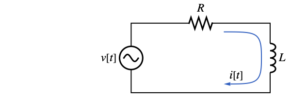
gf = GreenFunction[{circ, i[0] == 0}, i[t], {t, 0, ∞}, s]Find the current for a given voltage source:
v[t_] := Sin[ω t]Integrate[v[s] gf, {s, 0, t}, Assumptions -> t > 0]Plot[% /. {L -> 2, R -> 1, ω -> 5}, {t, 0, 10}]Compute the displacement u[x] for a string of length p and tension T that is fixed at the two ends and is subjected to a force per unit length of f[x]. The operator for the displacement is given by:
strop = T u''[x];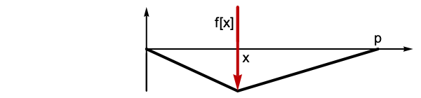
gf = GreenFunction[{strop, u[0] == 0, u[p] == 0}, u[x], {x, 0, p}, y]Find the displacement for a given force:
f[x_] := x ^ 2(x - p)Integrate[f[y] gf, {y, 0, p}, Assumptions -> p > 0 && 0 < x < p]Plot[% /. {T -> 3, p -> 5}, {x, 0, 5}]The impulse response of a continuous linear time-invariant system can be found by using the Green's function for the system with homogeneous initial conditions. Compute the impulse response for the system defined by:
sys = 2y''[t] + 8y'[t] + 6y[t];Green's function for the system with homogeneous initial conditions:
gf = GreenFunction[{sys, y[0] == 0, y'[0] == 0}, y[t], {t, 0, ∞}, s]Obtain the impulse response by setting s=0:
ir = gf /. {s -> 0}Plot[ir, {t, -3, 7}]Properties & Relations (2)
Compute a Green's function for a differential equation:
GreenFunction[{u'[x] + u[x], u[0] == 0}, u[x], {x, 0, ∞}, y]Obtain the same result using DSolve:
DSolve[{u'[x] + u[x] == DiracDelta[x - y], u[0] == 0}, u[x], x, Assumptions -> y > 0]GreenFunction is related to OutputResponse and TransferFunctionModel:
GreenFunction[{u''[t] + 3u'[t] + 2u[t], u[0] == 0}, u[t], {t, 0, ∞}, 0]Simplify[OutputResponse[TransferFunctionModel[{{{1}}, 2 + 3*s + s^2}, s], DiracDelta[t], t][[1]]]Text
Wolfram Research (2016), GreenFunction, Wolfram Language function, https://reference.wolfram.com/language/ref/GreenFunction.html.
CMS
Wolfram Language. 2016. "GreenFunction." Wolfram Language & System Documentation Center. Wolfram Research. https://reference.wolfram.com/language/ref/GreenFunction.html.
APA
Wolfram Language. (2016). GreenFunction. Wolfram Language & System Documentation Center. Retrieved from https://reference.wolfram.com/language/ref/GreenFunction.html