HjorthDistribution

HjorthDistribution[m,s,f]

位置母数 m，尺度母数 s，形状母数 f のHjorth分布を表す．

詳細

HjorthDistributionは，信頼性解析における故障のさまざまなクラスのモデル化に適用されてきた分布である．
Hjorth分布における値についての生存関数は，については，それ以外の場合はである．
HjorthDistribution[m,s,f]の m および s は任意の正の実数でよく，f は任意の非負の実数でよい．
HjorthDistribution[m,s,f]の m，s および f は，m*s および m*f が無次元となる任意の数量でよい． »
HjorthDistributionは，Mean，CDF，RandomVariate等の関数で使うことができる．

例題

すべて開くすべて閉じる

例 (3)

さまざまな母数値についての確率密度関数：

Wolfram Language code:

Plot[Table[PDF[HjorthDistribution[.8, 4, f], x], {f, {0.1, 0.5, 1.2}}]//Evaluate, {x, 0, 3}, PlotRange -> All, Filling -> Axis]

Wolfram Language code:

Plot[Table[PDF[HjorthDistribution[m, 8, 1], x], {m, {0.1, 0.5, 1.2}}]//Evaluate, {x, 0, 1}, PlotRange -> All, Filling -> Axis]

Wolfram Language code: PDF[HjorthDistribution[m, s, f], x]

さまざまな母数値についての累積分布関数：

Wolfram Language code: Plot[Table[CDF[HjorthDistribution[.8, .1, f], x], {f, {0.1, 0.5, 1.2}}]//Evaluate, {x, 0, 3}, Filling -> Axis]

Wolfram Language code:

Plot[Table[CDF[HjorthDistribution[m, 8, 1], x], {m, {0.1, 0.5, 1.2}}]//Evaluate, {x, 0, 3}, PlotRange -> All, Filling -> Axis]

Wolfram Language code: CDF[HjorthDistribution[m, s, f], x]

平均：

Wolfram Language code: Mean[HjorthDistribution[m, s, f]]

分散は数値で得られる：

Wolfram Language code: Variance[HjorthDistribution[2, 47, 1 / 3]]

Wolfram Language code: N[%]

スコープ (6)

Hjorth分布の擬似乱数のサンプルを生成する：

Wolfram Language code: data = RandomVariate[HjorthDistribution[2, 3, 0.1], 10 ^ 4];

そのヒストグラムを確率密度関数と比較する：

Wolfram Language code:

Show[Histogram[data, {0, 10, 0.5}, "PDF"], 
	Plot[PDF[HjorthDistribution[2, 3, 0.1], x], {x, 0, 10}, PlotStyle -> Thick]]

分布母数推定：

Wolfram Language code: sample = RandomVariate[HjorthDistribution[4, 7, 0.5], 10 ^ 3];

サンプルデータから分布母数を推定する：

Wolfram Language code: edist = EstimatedDistribution[sample, HjorthDistribution[4, 7, f]]

サンプルの密度ヒストグラムを推定分布の確率密度関数と比較する：

Wolfram Language code: Show[Histogram[sample, {0, 10, 0.5}, "PDF"], Plot[PDF[edist, x], {x, 0, 10}, PlotStyle -> Thick]]

母数の関数としての閉じた形の種々のモーメント：

Wolfram Language code: FormulaGrid[list_, type_] := Grid[...]

Moment：

Wolfram Language code: FormulaGrid[Table[Moment[HjorthDistribution[m, s, f], k], {k, 3}], M]

記号次数の閉じた形：

Wolfram Language code: Moment[HjorthDistribution[m, s, f], r]

CentralMoment：

Wolfram Language code: FormulaGrid[Table[CentralMoment[HjorthDistribution[m, s, f], k], {k, 3}], CM]

FactorialMoment：

Wolfram Language code: FormulaGrid[Table[FactorialMoment[HjorthDistribution[m, s, f], k], {k, 3}], M]

Cumulant：

Wolfram Language code: FormulaGrid[Table[Cumulant[HjorthDistribution[m, s, f], k], {k, 3}], CM]

ハザード関数：

Wolfram Language code: Plot[Table[HazardFunction[HjorthDistribution[m, 1, 5], x], {m, {0.7, 1.4, 4}}]//Evaluate, {x, 0, 10}, Filling -> Axis]

Wolfram Language code: Plot[Table[HazardFunction[HjorthDistribution[3, s, 5], x], {s, {0.1, 1, 10}}]//Evaluate, {x, 0, 10}, Filling -> Axis]

Wolfram Language code: Plot[Table[HazardFunction[HjorthDistribution[3, 2, f], x], {f, {0.1, 1, 3}}]//Evaluate, {x, 0, 10}, Filling -> Axis]

Wolfram Language code: HazardFunction[HjorthDistribution[m, s, f], x]

分位関数：

Wolfram Language code: Plot[Table[Quantile[HjorthDistribution[2, 5, f], q], {f, {2, 3, 6}}]//Evaluate, {q, 0, 1}, Filling -> Axis]

母数で一定してQuantityを使うとQuantityDistributionが与えられる：

Wolfram Language code: lifetime𝒟 = HjorthDistribution[Quantity[98.3, "Months"], Quantity[41, 1 / "Months"], Quantity[4.5, 1 / "Months"]]

時間の中央値求める：

Wolfram Language code: Median[lifetime𝒟]

アプリケーション (5)

寿命がHjorthDistributionに従うデバイスがある．このデバイスの信頼性を求める：

Wolfram Language code: SurvivalFunction[HjorthDistribution[m, s, f], t]

平均寿命を求める：

Wolfram Language code: Mean[HjorthDistribution[m, s, f]]

ハザード率の可能な形状をプロットする：

Wolfram Language code: hf[m_, s_, f_] := HazardFunction[HjorthDistribution[m, s, f], t]

Wolfram Language code:

bathtub = hf[2, 5, 2];
incr = hf[1.7, 1 / 7, 2];
decr = Limit[hf[m, 2, 2], m -> Infinity];
const = Limit[Limit[hf[m, s, 2], m -> Infinity], s -> 0];

Wolfram Language code: Plot[{bathtub, incr, decr, const}, {t, 0, 8}, PlotLegends -> {"bathtub", "increasing", "decreasing", "constant"}]

ある部品の故障は，母数が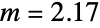，，のHjorthDistributionで説明することができる．この部品が最初の1年以内に故障する確率を求める：

Wolfram Language code: 𝒟 = QuantityDistribution[HjorthDistribution[2.17, 9.03, 0.17], "Years"];

Wolfram Language code: Probability[x ≤ Quantity[1, "Year"], x𝒟]

故障時の密度関数をプロットする：

Wolfram Language code: Plot[PDF[𝒟, Quantity[t, "Years"]], {t, 0, 8}, Filling -> Axis]

この部品が最も故障しそうな時間を求める：

Wolfram Language code: Quantity[First@FindArgMax[QuantityMagnitude@PDF[𝒟, Quantity[t, "Years"]], t], "Years"]

故障までの平均時間を求める：

Wolfram Language code: Mean[𝒟]

この部品が90%の安全性で故障を免れるのはどのくらいの期間であるかを求める：

Wolfram Language code: InverseSurvivalFunction[𝒟, 0.9]

この部品が2年の後にもう1年故障を免れる確率を求める：

Wolfram Language code: NProbability[x ≥ Quantity[3, "Years"]x ≥ Quantity[2, "Years"], x𝒟]

これと類似する独立した30個の部品の故障時のシミュレーションを行う：

Wolfram Language code:

ListPlot[{RandomVariate[𝒟, 30], {{0, Mean[𝒟]}, {30, Mean[𝒟]}}}, Joined -> {False, True}, Filling -> Axis, AxesLabel -> Automatic]

生産過程における品質変化のランダム性のために，ある電子装置の部品は初期故障率が高くなっている．この部品の寿命は，母数が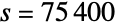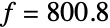，，のHjorthDistributionでモデル化できる．ハザード関数をプロットする：

Wolfram Language code: 𝒟 = QuantityDistribution[HjorthDistribution[6, 75400, 800.8], "Years"];

Wolfram Language code: Plot[HazardFunction[𝒟, Quantity[t, "Years"]], {t, 0, 2}, Filling -> Axis]

平均寿命：

Wolfram Language code: Mean[𝒟]

1年目（保証期間）の故障確率：

Wolfram Language code: Probability[t ≤ Quantity[1, "Year"], t𝒟]

早い時期の故障を避けるため，この装置は「バーンイン」期間中は応力水準で運転される．期間後は1年目の故障確率が半減する「バーンイン」期間を求める：

Wolfram Language code:

eqn = (CDF[𝒟, Quantity[1, "Years"] + Quantity[bp, "Years"]] - CDF[𝒟, Quantity[bp, "Years"]]) / (1 - CDF[𝒟, Quantity[bp, "Years"]]) == CDF[𝒟, Quantity[1, "Years"]] / 2;

Wolfram Language code: Solve[{eqn, 0 < bp < 1}, bp]//Quiet

Wolfram Language code: burnIn = Quantity[bp /. First[%], "Years"]

Wolfram Language code: UnitConvert[burnIn, "Days"]

「バーンイン」期間に故障を免れた後の，この装置の期待される寿命を求める：

Wolfram Language code: NExpectation[tt ≥ burnIn, t𝒟]

この装置の信頼性が最も高くなる時を求める：

Wolfram Language code: maxRel = Quantity[ArgMin[{HazardFunction[𝒟, Quantity[t, "Years"]], t > 0}, t], "Years"]

これと類似した装置の独立した50の部品について故障時のシミュレーションを行う：

Wolfram Language code:

ListPlot[{RandomVariate[𝒟, 50], {{0, Mean[𝒟]}, {50, Mean[𝒟]}}, {{0, maxRel}, {50, maxRel}}}, Joined -> {False, True, True}, Filling -> Axis, AxesLabel -> Automatic, PlotLegends -> {"Simulated", "Mean", "'Infant mortality' zone"}]

独立した3つの部品からなる比較的単純な機械系がある．部品の2つはタイプAで1つはタイプBである．測定された故障時（単位：日）は次のようになる：

Wolfram Language code:

compA = WeightedData[Automatic, {{2.981404513903204, 0.5168657254928053, 4.817574310667597, 
   2.251404494427119, 2.600964244987795, 3.9249944934780108, 4.692482778918926, 2.573280108286907, 
   3.986933723430509, 4.06761198577694, 4.521085806658003, 6.70 ...  1, 1, 1, 1, 1, 1, 1, 1, 1, 1, 1, 1, 1, 1, 1, 1, 1, 1, 1, 1, 1, 1, 1, 1, 1, 
   1, 1, 1, 1, 1, 1, 1, 1, 1, 1, 1, 1, 1, 1, 1, 1, 1, 1, 1, 1, 1, 1, 1, 1, 1, 1, 1, 1, 1, 1, 1, 1, 
   1, 1, 1, 1, 1, 1, 1, 1, 1, 1, 1, 1, 1, 1, 1, 1, 1, 1, 1, 1, 1, 1}}];
compB = WeightedData[Automatic, {{30.325585961084265, 27.513700329498764, 28.010248120775593, 
   10.90353777134251, 27.52007434803306, 46.19838803147495, 56.50179419020349, 35.98911572744762, 
   47.62033758291881, 49.76020651274327, 82.22210996662847, 35 ...  1, 1, 1, 1, 1, 1, 1, 1, 1, 1, 1, 1, 1, 1, 1, 1, 1, 1, 1, 1, 1, 1, 1, 1, 1, 
   1, 1, 1, 1, 1, 1, 1, 1, 1, 1, 1, 1, 1, 1, 1, 1, 1, 1, 1, 1, 1, 1, 1, 1, 1, 1, 1, 1, 1, 1, 1, 1, 
   1, 1, 1, 1, 1, 1, 1, 1, 1, 1, 1, 1, 1, 1, 1, 1, 1, 1, 1, 1, 1, 1}}];

HjorthDistributionを仮定して，両方の部品についての推定分布を求める：

Wolfram Language code: estimateA = EstimatedDistribution[compA, HjorthDistribution[m, s, f]]

Wolfram Language code: estimateB = EstimatedDistribution[compB, HjorthDistribution[m, s, f]]

各部品の故障時の分布をデータと比較する：

Wolfram Language code:

Show[Histogram[{compA, compB}, 20, "PDF"], Plot[{PDF[estimateB, t], PDF[estimateA, t]}, {t, 0, 90}, PlotRange -> All, PlotStyle -> Thick, PlotLegends -> {"B", "A"}]]

この系は，各タイプの部品が1つずつ動いていれば稼働する．この系の信頼性を求める：

Wolfram Language code:

dist = ReliabilityDistribution[(Subscript[a, 1]∨Subscript[a, 2])∧b, {{Subscript[a, 1], estimateA}, {Subscript[a, 2], estimateA}, {b, estimateB}}];

Wolfram Language code: Plot[SurvivalFunction[dist, t], {t, 0, 10}, Filling -> Axis]

故障までの平均時間を求める：

Wolfram Language code: Mean[dist]

この系が3日目以降に故障する確率を求める：

Wolfram Language code: Probability[t <= 3, tdist]

独立した3つの部品からなる比較的単純な機械系がある．部品の2つはタイプAで1つはタイプBである．この系は，各タイプの部品が1つずつ動いていれば稼働する．各部品の故障時は次の分布に従う：

Wolfram Language code:

distA = QuantityDistribution[HjorthDistribution[2.7, 1.34, 0.001], "Days"];
distB = QuantityDistribution[HjorthDistribution[31, 0.02, 0.002], "Days"];

タイプBの部品が故障する前にタイプAの部品が両方とも故障する確率を求める：

Wolfram Language code: NProbability[a1 < b∧a2 < b, {a1distA, a2distA, bdistB}]

タイプAの部品は，故障するたびにすぐに交換される．タイプBの部品が故障する前に必要となるタイプAの部品の平均数を求める：

Wolfram Language code: Floor[2Mean[distB] / Mean[distA]]

タイプAの部品数を増やした場合の，この系の期待される寿命：

Wolfram Language code:

distExt[j_] := ReliabilityDistribution[Or@@Table[Subscript[a, i], {i, j}]∧b, Table[{Subscript[a, i], distA}, {i, j}]~Join~{{b, distA}}];

Wolfram Language code: means = Table[{j, Mean[distExt[j]]}, {j, 2, 10}];

Wolfram Language code:

Grid[Prepend[means, {"# of components A", "Expected lifetime"}], Alignment -> Bottom, Frame -> All, Background -> {{None, None}, {LightGray, None}}]

結果をプロットする：

Wolfram Language code: ListPlot[means, Filling -> Axis, AxesLabel -> Automatic]

特性と関係 (5)

Hjorth分布は，正の因数によるスケーリングの下では閉じている：

Wolfram Language code: TransformedDistribution[k * u, uHjorthDistribution[m, s, f]]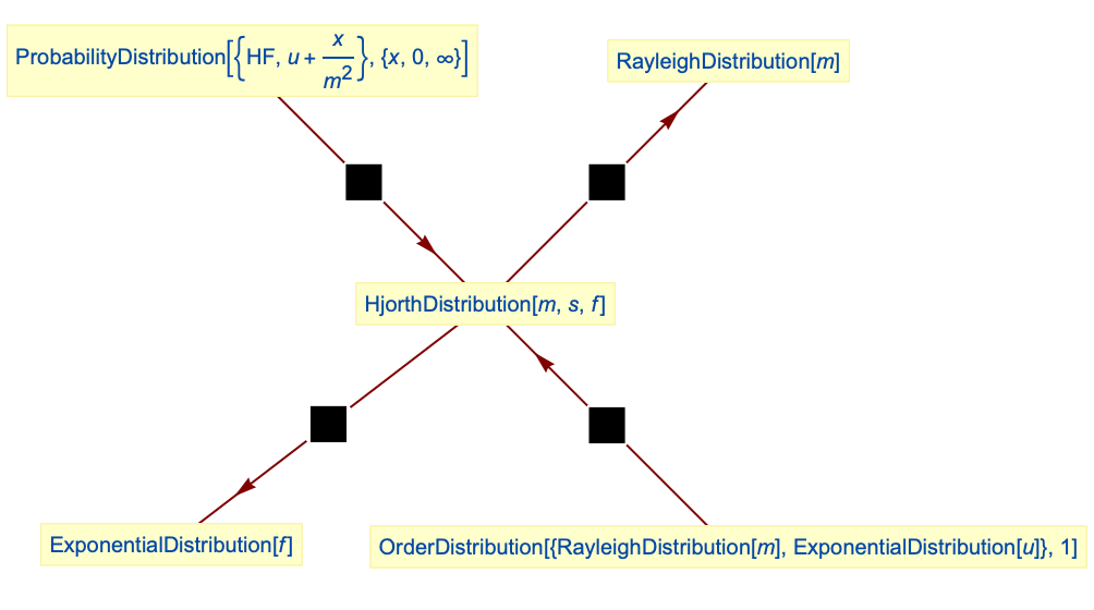

他の分布との関係：

Hjorth分布を簡約するとRayleighDistributionになる：

Wolfram Language code: PDF[HjorthDistribution[m, s, 0], x]

Wolfram Language code: PDF[RayleighDistribution[m], x]

Wolfram Language code: Simplify[% - %%]

Hjorth分布は，初期故障率がGammaDistributionに従う線形ハザード率のParameterMixtureDistributionとして得ることができる：

Wolfram Language code: lhr[u_, m_] := ProbabilityDistribution[{"HF", u + x / m ^ 2}, {x, 0, ∞}]

Wolfram Language code: 𝒟 = ParameterMixtureDistribution[lhr[u, m], uGammaDistribution[f / s, s]];

Wolfram Language code: CDF[𝒟, x]

Wolfram Language code: CDF[HjorthDistribution[m, s, f], x]

Wolfram Language code: Simplify[% - %%]

線形ハザード率分布は，ExponentialDistributionおよびRayleighDistributionのOrderDistributionとして得ることができる：

Wolfram Language code: distOrd = OrderDistribution[{RayleighDistribution[m], ExponentialDistribution[u]}, 1];

Wolfram Language code: Simplify[PDF[lhr[u, m], x] - PDF[distOrd, x], Assumptions -> x > 0]

ExponentialDistributionはHjorth分布の極限ケースである：

Wolfram Language code: Limit[Limit[PDF[HjorthDistribution[m, s, f], x], s -> 0], m -> ∞]

Wolfram Language code: PDF[ExponentialDistribution[f], x]

Wolfram Language code: Simplify[% - %%]

考えられる問題 (5)

HjorthDistributionは，m あるいは s が正の実数でなければ定義されない：

Wolfram Language code: Mean[HjorthDistribution[3 + I, 1, 2]]

HjorthDistributionは，f が非負の実数ではない場合は定義されない：

Wolfram Language code: Mean[HjorthDistribution[3, 1, -2]]

記号出力に無効なパラメータを代入すると，意味のない結果が与えられる：

Wolfram Language code: Mean[HjorthDistribution[m, s, f]] /. {m -> 2, s -> 1 - I, f -> -1}//N

Hjorth分布の特性関数は，閉じた形の表現を持たない：

Wolfram Language code: CharacteristicFunction[HjorthDistribution[m, s, f], t]

数値入力にすると関数の値を求めることができる：

Wolfram Language code: CharacteristicFunction[HjorthDistribution[1.3, 3.2, 4], .5]

Wolfram Language code: CharacteristicFunction[HjorthDistribution[13 / 10, 32 / 10, 4], 1 / 2]

Wolfram Language code: N[%]

Hjorth分布のモーメントの閉じた形を使うと，パラメータによっては数値的な不安定さを招くことがある：

Wolfram Language code: mom = Moment[HjorthDistribution[1, 1 / 10, 5], 10]

Wolfram Language code: N[%]

厳密ではないパラメータを使ってモーメントの数値近似を求める：

Wolfram Language code: Moment[HjorthDistribution[1, 0.1, 5], 10]

代りに，より高精度で閉じた式を評価することもできる：

Wolfram Language code: Block[{$MaxExtraPrecision = 100}, N[mom /. {m -> 1, s -> 1 / 10, f -> 5, r -> 10}, 16]//Re]

おもしろい例題 (1)

CDF等高線のある，sのさまざまな値についてのPDF：

Wolfram Language code:

dist = HjorthDistribution[1.3, s, 1 / 4];cdf = Function[{x, s}, Evaluate[CDF[dist, x]]];
ql = {0.025, 0.10, 0.25, 0.5, 0.75, 0.90, 0.975};
cl = Table[ColorData["Rainbow"][q], {q, Join[{0.0}, ql]}];

Wolfram Language code:

Legended[Plot3D[PDF[dist, x], {x, 0, 4}, {s, 0.01, 10}, PlotTheme -> "Marketing", MeshFunctions -> {cdf}, Mesh -> {ql}, MeshStyle -> GrayLevel[0.8], MeshShading -> cl, AxesLabel -> Automatic, BaseStyle -> Opacity[0.9], ImageSize -> 400, PlotRange -> All, PlotPoints -> 50], BarLegend["Rainbow", ql, LegendLabel -> "prob"]]

Top

その他のラーニングリソース

テクニカルサポート

データサイエンス，金融，ビジネス

工学

科学とテクノロジー

教育のためのテクノロジー

教育イニシアチブ

使い始める

Grow Your Skills

Wolframと繋がる

大人用の教育プログラム

若者のための教育プログラム

読む

HjorthDistribution

詳細

例題

例 (3)

スコープ (6)

アプリケーション (5)

特性と関係 (5)

考えられる問題 (5)

おもしろい例題 (1)

テキスト

CMS

APA

BibTeX

BibLaTeX

HjorthDistribution

詳細

例題

例 (3)

スコープ (6)

アプリケーション (5)

特性と関係 (5)

考えられる問題 (5)

おもしろい例題 (1)

関連項目

テクニカルノート

関連するガイド

履歴

テキスト

CMS

APA

BibTeX

BibLaTeX