


MassTransportPDEComponent
MassTransportPDEComponent[vars,pars]
yields a mass transport PDE term with variables vars and parameters pars.
Details
- MassTransportPDEComponent returns a sum of differential operators to be used as a part of partial differential equations:
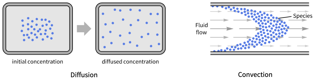
- MassTransportPDEComponent models the generation and propagation of diluted mass species in physical systems such as mixtures, solutions and solids by mechanisms of diffusion or convection.
- MassTransportPDEComponent models are applicable when the concentration of the diluted species is at least one order of magnitude less than the concentration of the solvent.
- MassTransportPDEComponent models mass transport phenomena with dependent variable
 in [
in [![TemplateBox[{InterpretationBox[, 1], {"mol", , "/", , {"m", ^, 3}}, moles per meter cubed, {{(, "Moles", )}, /, {(, {"Meters", ^, 3}, )}}}, QuantityTF]](Files/MassTransportPDEComponent.en/4.png "TemplateBox[{InterpretationBox[, 1], {\"mol\", , \"/\", , {\"m\", ^, 3}}, moles per meter cubed, {{(, \"Moles\", )}, /, {(, {\"Meters\", ^, 3}, )}}}, QuantityTF]") ], independent variables
], independent variables  in [
in [![TemplateBox[{InterpretationBox[, 1], "m", meters, "Meters"}, QuantityTF]](Files/MassTransportPDEComponent.en/6.png "TemplateBox[{InterpretationBox[, 1], \"m\", meters, \"Meters\"}, QuantityTF]") ] and time variable
] and time variable  in [
in [![TemplateBox[{InterpretationBox[, 1], "s", seconds, "Seconds"}, QuantityTF]](Files/MassTransportPDEComponent.en/8.png "TemplateBox[{InterpretationBox[, 1], \"s\", seconds, \"Seconds\"}, QuantityTF]") ].
]. - Stationary variables vars are vars={c[x1,…,xn],{x1,…,xn}}.
- Time-dependent variables vars are vars={c[t,x1,…,xn],t,{x1,…,xn}}.
- MassTransportPDEComponent provides both a conservative model to be used with compressible fluids and a non-conservative model to be used with incompressible fluids.
- The non-conservative time-dependent mass transport model MassTransportPDEComponent is based on a convection-diffusion model with mass diffusivity
 , mass convection velocity vector
  , mass reaction rate
  and mass source term
  :
: - The conservative time-dependent mass transport model MassTransportPDEComponent is based on a conservative convection-diffusion model given by:
- The non-conservative stationary mass transport PDE term is given by:
- The implicit default boundary condition for the non-conservative model is a MassOutflowValue.
- The conservative stationary mass transport PDE term is given by:
- The implicit default boundary condition for the conservative model is a MassImpermeableBoundaryValue.
- The difference between the non-conservative and the conservative models is the treatment of a convection velocity
 .
. - The non-conservative model is the default model. The conservative model should be used when the divergence of convection velocity
 is nonzero.
 - The units of the mass transport PDE terms are in [
![TemplateBox[{InterpretationBox[, 1], {"mol", , "/(", , {"m", ^, 3}, , "s", , ")"}, moles per meter cubed second, {{(, "Moles", )}, /, {(, {{"Meters", ^, 3}, , "Seconds"}, )}}}, QuantityTF]](Files/MassTransportPDEComponent.en/19.png "TemplateBox[{InterpretationBox[, 1], {\"mol\", , \"/(\", , {\"m\", ^, 3}, , \"s\", , \")\"}, moles per meter cubed second, {{(, \"Moles\", )}, /, {(, {{\"Meters\", ^, 3}, , \"Seconds\"}, )}}}, QuantityTF]") ].
]. - The following model parameters pars can be given:
-
parameter default symbol "MassConvectionVelocity" 
 , flow velocity [
![TemplateBox[{InterpretationBox[, 1], {"m", , "/", , "s"}, meters per second, {{(, "Meters", )}, /, {(, "Seconds", )}}}, QuantityTF]](Files/MassTransportPDEComponent.en/22.png "TemplateBox[{InterpretationBox[, 1], {\"m\", , \"/\", , \"s\"}, meters per second, {{(, \"Meters\", )}, /, {(, \"Seconds\", )}}}, QuantityTF]") ]
]"DiffusionCoefficient" IdentityMatrix  , mass diffusivity [
![TemplateBox[{InterpretationBox[, 1], {{"m", ^, 2}, , "/", , "s"}, meters squared per second, {{(, {"Meters", ^, 2}, )}, /, {(, "Seconds", )}}}, QuantityTF]](Files/MassTransportPDEComponent.en/24.png "TemplateBox[{InterpretationBox[, 1], {{\"m\", ^, 2}, , \"/\", , \"s\"}, meters squared per second, {{(, {\"Meters\", ^, 2}, )}, /, {(, \"Seconds\", )}}}, QuantityTF]") ]
]"MassReactionRate" 0  , mass reaction rate in [1/
![TemplateBox[{InterpretationBox[, 1], "s", seconds, "Seconds"}, QuantityTF]](Files/MassTransportPDEComponent.en/26.png "TemplateBox[{InterpretationBox[, 1], \"s\", seconds, \"Seconds\"}, QuantityTF]") ]
]"MassSource" 0  , mass source [
![TemplateBox[{InterpretationBox[, 1], {"mol", , "/(", , {"m", ^, 3}, , "s", , ")"}, moles per meter cubed second, {{(, "Moles", )}, /, {(, {{"Meters", ^, 3}, , "Seconds"}, )}}}, QuantityTF]](Files/MassTransportPDEComponent.en/28.png "TemplateBox[{InterpretationBox[, 1], {\"mol\", , \"/(\", , {\"m\", ^, 3}, , \"s\", , \")\"}, moles per meter cubed second, {{(, \"Moles\", )}, /, {(, {{\"Meters\", ^, 3}, , \"Seconds\"}, )}}}, QuantityTF]") ]
]"ModelForm" "NonConservative" 
"RegionSymmetry" None 
- All parameters may depend on any of
 ,
,  and
and  , as well as other dependent variables.
 - The number of independent variables
 determines the dimensions of
  and the length of
  .
. - The mass convection velocity specifies the velocity
 with which a fluid transports mass.
 - A mass reaction term
 models mass chemical reactions of masses.
 - A mass source
 models mass that is generated (positive) or absorbed (negative).
 - Possible choices for the parameter "ModelForm" are "Conservative" and "NonConservative".
- A possible choice for the parameter "RegionSymmetry" is "Axisymmetric".
- "Axisymmetric" region symmetry represents a truncated cylindrical coordinate system where the cylindrical coordinates are reduced by removing the angle variable as follows:
-
dimension reduction non-conservative equation 1D 

2D 

-
dimension reduction conservative equation 1D 

2D 

- The input specification for the parameters is exactly the same as for their corresponding operator terms.
- Coupled equations can be generated with the same input specification as with the corresponding operator terms.
- If no parameters are specified, the default mass transport PDE is:
- If the MassTransportPDEComponent depends on parameters
 that are specified in the association pars as …,keypi…,pivi,…, the parameters
  are replaced with
  .
.
Examples
open all close allBasic Examples (3)
Define a time-dependent mass transport model:
MassTransportPDEComponent[{c[t, x], t, {x}}, <||>]Set up a time-dependent mass transport model with particular material parameters:
MassTransportPDEComponent[{c[t, x], t, {x}}, <|"DiffusionCoefficient" -> d|>]Model a 1D chemical species field in an incompressible fluid whose right side and left side are subjected to a mass concentration and inflow condition, respectively:
Set up the stationary mass transport model variables vars:
vars = {c[x], {x}};Ω = Line[{{0}, {1}}];Specify the mass transport model parameters species diffusivity ![]() and fluid flow velocity
and fluid flow velocity ![]() :
:
pars = <|"DiffusionCoefficient" -> 0.026, "MassConvectionVelocity" -> {0.1}|>;Specify a species flux boundary condition:
Subscript[Γ, flux] = MassFluxValue[x == 0, vars, pars, <|"MassFlux" -> 1|>]Specify a mass concentration boundary condition:
Subscript[Γ, C] = MassConcentrationCondition[x == 1, vars, pars, <|"MassConcentration" -> 0|>]eqn = MassTransportPDEComponent[vars, pars] == Subscript[Γ, flux]cfun = NDSolveValue[{eqn, Subscript[Γ, C]}, c, x∈Ω];Plot[cfun[x], x∈Ω, Rule[...]]Scope (23)
Basic Usage (9)
Set up a time-dependent mass transport model with numeric material parameters:
MassTransportPDEComponent[{c[t, x], t, {x}}, <|"DiffusionCoefficient" -> 2|>]Define a 2D stationary mass transport model:
MassTransportPDEComponent[{c[x, y], {x, y}}, <|"DiffusionCoefficient" -> 1.2 * 10 ^ -6|>]Set up a 2D stationary mass transport model with an orthotropic mass diffusion:
MassTransportPDEComponent[{c[x, y], {x, y}}, <|"DiffusionCoefficient" -> {1, 2}|>]Set up a 2D stationary mass transport model with a diffusivity matrix:
MassTransportPDEComponent[{c[x, y], {x, y}}, <|"DiffusionCoefficient" -> IdentityMatrix[2]|>]Set up a 2D stationary mass transport model with an anisotropic diffusivity matrix:
MassTransportPDEComponent[{c[x, y], {x, y}}, <|"DiffusionCoefficient" -> {{2, 3}, {0, 4}}|>]Define a 2D stationary mass transport model with a material change:
MassTransportPDEComponent[{c[x, y], {x, y}}, <|"DiffusionCoefficient" -> If[x < 1 / 2, 1, 2] * IdentityMatrix[2]|>]Define a 2D stationary mass transport model with a material change and an anisotropic material:
MassTransportPDEComponent[{c[x, y], {x, y}}, <|"DiffusionCoefficient" -> If[x < 1 / 2, {{1, 0}, {0, 1}}, {{2, 1}, {0, 3}}]|>]Set up a coupled 2D stationary mass transport model:
MassTransportPDEComponent[{{c1[x, y], c2[x, y]}, {x, y}}, <|"DiffusionCoefficient" -> {{1, 10 ^ -3}, {2 * 10 ^ -3, 1}}|>]Set up a coupled 2D transient mass transport model with cross-coupled nonlinear reaction terms:
MassTransportPDEComponent[{{c1[t, x, y], c2[t, x, y]}, t, {x, y}}, <|"DiffusionCoefficient" -> {{1, 10 ^ -3}, {2 * 10 ^ -3, 1}}, "MassReactionRate" -> {{c1[t, x, y] * c2[t, x, y], c1[t, x, y]}, {0, Sqrt[c1[t, x, y]]}}|>]1D (1)
Model a 1D chemical species field in an incompressible fluid whose right side and left side are subjected to a mass concentration and inflow condition, respectively:
Set up the stationary mass transport model variables vars:
vars = {c[x], {x}};Ω = Line[{{0}, {1}}];Specify the mass transport model parameters species diffusivity ![]() and fluid flow velocity
and fluid flow velocity ![]() :
:
pars = <|"DiffusionCoefficient" -> 0.026, "MassConvectionVelocity" -> {0.1}|>;Specify a species flux boundary condition:
Subscript[Γ, flux] = MassFluxValue[x == 0, vars, pars, <|"MassFlux" -> 1|>]Specify a mass concentration boundary condition:
Subscript[Γ, C] = MassConcentrationCondition[x == 1, vars, pars, <|"MassConcentration" -> 0|>]eqn = MassTransportPDEComponent[vars, pars] == Subscript[Γ, flux]cfun = NDSolveValue[{eqn, Subscript[Γ, C]}, c, x∈Ω];Plot[cfun[x], x∈Ω, Rule[...]]1D Axisymmetric (3)
Define a 1D axisymmetric stationary mass transport model:
MassTransportPDEComponent[{c[r], {r}}, <|"DiffusionCoefficient" -> {{d}}, "MassConvectionVelocity" -> {Subscript[v, r]}, "RegionSymmetry" -> "Axisymmetric"|>]Define a 1D axisymmetric conservative stationary mass transport model:
MassTransportPDEComponent[{c[r], {r}}, <|"DiffusionCoefficient" -> {{d}}, "MassConvectionVelocity" -> {Subscript[v, r]}, "RegionSymmetry" -> "Axisymmetric", "ModelForm" -> "Conservative"|>]lammEquation = MassTransportPDEComponent[{c[t, r], t, {r}}, <|"DiffusionCoefficient" -> {{d}}, "RegionSymmetry" -> "Axisymmetric", "MassConvectionVelocity" -> {sc ω ^ 2 r}, "ModelForm" -> "Conservative"|>] == 0Look at the activated and simplified form of the equation:
Simplify[Activate[lammEquation]]2D (2)
Model mass transport of a pollutant in a 2D rectangular region in an isotropic homogeneous medium. Initially, the pollutant concentration is zero throughout the region of interest. A concentration of 3000 ![]() is maintained at a strip with dimension 0.2
is maintained at a strip with dimension 0.2 ![]() located at the center of the left boundary, while the right boundary is subject to a parallel species flow with a constant concentration of 1500
located at the center of the left boundary, while the right boundary is subject to a parallel species flow with a constant concentration of 1500 ![]() , allowing for mass transfer. A pollutant outflow of 100
, allowing for mass transfer. A pollutant outflow of 100 ![]() is applied at both the top and bottom boundaries. A diffusion coefficient of 0.833
is applied at both the top and bottom boundaries. A diffusion coefficient of 0.833 ![]() is distributed uniformly with a uniform horizontal velocity of 0.01
is distributed uniformly with a uniform horizontal velocity of 0.01 ![]() :
:
Set up the mass transport model variables vars:
vars = {c[x, y], {x, y}};Set up a rectangular domain with a width of ![]() and a height of
and a height of ![]() :
:
Ω = Rectangle[{0, 0}, {20, 10}];Specify model parameters species diffusivity ![]() and fluid flow velocity
and fluid flow velocity ![]() :
:
pars = <|"DiffusionCoefficient" -> 0.833, "MassConvectionVelocity" -> {0.01, 0}|>;Set up a species concentration source of 0.2 ![]() in length at the center of the left surface:
in length at the center of the left surface:
Subscript[Γ, concentration] = MassConcentrationCondition[x == 0 && y ≤ 5.1 && y ≥ 4.9, vars, pars, <|"MassConcentration" -> 3000|>]Set up a mass transfer boundary on the right surface:
Subscript[Γ, transfer] = MassTransferValue[x == 20, vars, pars, <|"AmbientConcentration" -> 1500, "MassTransferCoefficient" -> 5|>]Set up an outflow flux ![]() of
of ![]() on the top and bottom surfaces:
on the top and bottom surfaces:
Subscript[Γ, flux] = MassFluxValue[y == 0 || y == 10, vars, pars, <|"MassFlux" -> -100|>]eqn = MassTransportPDEComponent[vars, pars] == Subscript[Γ, transfer] + Subscript[Γ, flux]cfun = NDSolveValue[{eqn, Subscript[Γ, concentration]}, c, {x, y}∈Ω];ContourPlot[cfun[x, y], {x, y}∈Ω, ...]Symmetry boundaries can be used to reduce the size of the geometry of the model. Set up a mass transport equation:
vars = {c[x, y], {x, y}};
pars = <|"DiffusionCoefficient" -> 1, "MassSource" -> 1|>;
Set up and visualize a region:
Ω = RegionDifference[Rectangle[{-1, 0}, {1, 1}], Rectangle[{-1 / 2, 0}, {1 / 2, 1 / 2}]];
RegionPlot[Ω, AspectRatio -> Automatic]
Solve and visualize the equation:
cfun = NDSolveValue[{MassTransportPDEComponent[vars, pars] == 0, MassConcentrationCondition[y == 0, vars, pars, <|"MassConcentration" -> 0|>]}, c[x, y], {x, y}∈Ω];
ContourPlot[cfun, {x, y}∈Ω]
Set up a region about the symmetry axis at ![]() :
:
Ω = RegionDifference[Rectangle[{0, 0}, {1, 1}], Rectangle[{0, 0}, {1 / 2, 1 / 2}]];
Show[Graphics[{{Dashed, Thick, Gray, Line[{{0, -0.1}, {0, 1.1}}]}}], RegionPlot[Ω, AspectRatio -> Automatic]]
Solve and visualize the equation with a symmetry boundary at ![]() :
:
cfun = NDSolveValue[{MassTransportPDEComponent[vars, pars] == MassSymmetryValue[x == 0, vars, pars], MassConcentrationCondition[y == 0, vars, pars, <|"MassConcentration" -> 0|>]}, c[x, y], {x, y}∈Ω];
ContourPlot[cfun, {x, y}∈Ω]
2D Axisymmetric (2)
Define a 2D axisymmetric stationary mass transport model:
MassTransportPDEComponent[{c[r, z], {r, z}}, <|"DiffusionCoefficient" -> d * IdentityMatrix[2], "MassConvectionVelocity" -> {Subscript[v, r], Subscript[v, z]}, "RegionSymmetry" -> "Axisymmetric"|>]Define a 2D axisymmetric conservative stationary mass transport model:
MassTransportPDEComponent[{c[r, z], {r, z}}, <|"DiffusionCoefficient" -> d * IdentityMatrix[2], "MassConvectionVelocity" -> {Subscript[v, r], Subscript[v, z]}, "RegionSymmetry" -> "Axisymmetric", "ModelForm" -> "Conservative"|>]3D (1)
Model a non-conservative chemical species field in a unit cubic domain, with two mass conditions at two lateral surfaces and a mass inflow through a circle with radius 0.2 ![]() at the center of the top surface, as well as an orthotropic mass diffusivity
at the center of the top surface, as well as an orthotropic mass diffusivity ![]() :
:
Set up the mass transport model variables vars:
vars = {c[x, y, z], {x, y, z}};Ω = Cuboid[{0, 0, 0}, {1, 1, 1}];Specify a diffusivity ![]() and a flow velocity field
and a flow velocity field ![]() :
:
pars = <|"DiffusionCoefficient" -> {{1, 0, 0}, {0, 5, 0}, {0, 0, 10}}, "MassConvectionVelocity" -> {0, 10, 0}|>;Subscript[Γ, CC] = {MassConcentrationCondition[x == 0, vars, <|"MassConcentration" -> 0|>], MassConcentrationCondition[x == 1, vars, <|"MassConcentration" -> 1|>]}Specify a flux condition ![]() of
of ![]() through a regional circle on the top surface:
through a regional circle on the top surface:
Subscript[Γ, flux] = MassFluxValue[z == 1 && (x - 0.5) ^ 2 + (y - 0.5) ^ 2 ≤ 0.04, vars, pars, <|"MassFlux" -> 100|>]eqn = MassTransportPDEComponent[vars, pars] == Subscript[Γ, flux]cfun = NDSolveValue[{eqn, Subscript[Γ, CC]}, c, {x, y, z}∈Ω];GraphicsRow[Table[SliceContourPlot3D[cfun[x, y, z], sl, {x, y, z}∈Ω, ...], {...}]]Material Regions (1)
Model a 1D chemical species transport through different material with a reaction rate in one. The right side and left side are subjected to a mass concentration and inflow condition, respectively:
Set up the stationary mass transport model variables vars:
vars = {c[x], {x}};Ω = Line[{{0}, {1}}];Specify the mass transport model parameters species diffusivity ![]() and a reaction rate
and a reaction rate ![]() active in the region
active in the region ![]() :
:
pars = <|"DiffusionCoefficient" -> 0.01, "MassReactionRate" -> If[x > 1 / 2, 1, 0]|>;Specify a species flux boundary condition:
Subscript[Γ, flux] = MassFluxValue[x == 0, vars, pars, <|"MassFlux" -> 1|>]Specify a mass concentration boundary condition:
Subscript[Γ, C] = MassConcentrationCondition[x == 1, vars, pars, <|"MassConcentration" -> 0|>]eqn = MassTransportPDEComponent[vars, pars] == Subscript[Γ, flux]cfun = NDSolveValue[{eqn, Subscript[Γ, C]}, c, x∈Ω];Show[Plot[cfun[x], x∈Ω, Rule[...]], Graphics[...]]Time Dependent (1)
Model a 1D non-conservative chemical species field and a mass flux through part of the boundary with:
Set up the time-dependent mass transport model variables vars:
vars = {c[t, x], t, {x}};Ω = Line[{{0}, {1}}];Specify the mass transport model parameters mass diffusivity ![]() and mass convection velocity
and mass convection velocity ![]() :
:
pars = <|"DiffusionCoefficient" -> 0.01, "MassConvectionVelocity" -> {0.02}|>;Set up the equation with a mass flux ![]() of
of ![]() at the left end for the first 50 seconds:
at the left end for the first 50 seconds:
model = MassTransportPDEComponent[vars, pars] == MassFluxValue[x == 0, vars, pars, <|"MassFlux" -> Piecewise[{{10, t ≤ 50}, {0, t > 50}}]|>]Solve the PDE with an initial condition of a zero concentration:
cfun = NDSolveValue[{model, c[0, x] == 0}, c, {t, 0, 100}, x∈Ω];Manipulate[Show[Plot[cfun[t, x], ...], Graphics[...]], {{t, 30}, 0, 100, 2.5}, Rule[...]]Nonlinear Time Dependent (1)
Model a 1D non-conservative chemical species field with a nonlinear diffusivity coefficient ![]() and an outflow condition through part of the boundary, which is expressed as follows:
and an outflow condition through part of the boundary, which is expressed as follows:
Set up the mass transport model variables vars:
vars = {c[t, x], t, {x}};Ω = Line[{{0}, {1}}];Specify the nonlinear species diffusivity ![]() and fluid flow velocity
and fluid flow velocity ![]() :
:
pars = <|"DiffusionCoefficient" -> {{0.001 * Log[c[t, x] ^ 2 + 1]}}, "MassConvectionVelocity" -> {0.02}|>;Specify an outflow flux ![]() of
of ![]() applied at the right end:
applied at the right end:
Subscript[Γ, flux] = MassFluxValue[x == 1, vars, pars, <|"MassFlux" -> -1|>]Specify a time-dependent mass concentration surface condition:
Subscript[Γ, C] = MassConcentrationCondition[x == 0, vars, pars, <|"MassConcentration" -> 100 + 0.1 * t|>]ics = c[0, x] == 100;eqn = MassTransportPDEComponent[vars, pars] == Subscript[Γ, flux]cfun = NDSolveValue[{eqn, ics, Subscript[Γ, C]}, c, {t, 0, 500}, x∈Ω];Manipulate[Show[Plot[cfun[t, x], ...], Graphics[...]], {{t, 30}, 0, 500, 1}, Rule[...]]Coupled Time Dependent (2)
Model a 1D coupled non-conservative dual chemical species field with corresponding mass flux through the left parts of the boundary:
Set up the time-dependent mass transport model variables vars for the ![]() and
and ![]() species, respectively:
species, respectively:
vars = {{Subscript[c, 1][t, x], Subscript[c, 2][t, x]}, t, {x}};Ω = Line[{{0}, {1}}];Specify the mass transport model parameters mass diffusivity ![]() and
and ![]() for the
for the ![]() and
and ![]() species:
species:
pars = <|"DiffusionCoefficient" -> {{0.01, 0}, {0, 0.02}}|>;Set up the boundary conditions with a mass flux ![]() of 4
of 4 ![]() and 8
and 8 ![]() for
for ![]() and
and ![]() at the left end for the first 50 seconds:
at the left end for the first 50 seconds:
Subscript[Γ, flux] = MassFluxValue[x == 0, vars, pars, <|"MassFlux" -> {If[t ≤ 50, 4, 0], If[t ≤ 50, 8, 0]}|>]eqn = MassTransportPDEComponent[vars, pars] == Subscript[Γ, flux]ics = {Subscript[c, 1][0, x] == 0, Subscript[c, 2][0, x] == 0};{c1fun, c2fun} = NDSolveValue[{eqn, ics}, {Subscript[c, 1], Subscript[c, 2]}, {t, 0, 100}, {x}∈Ω];Manipulate[Show[Plot[{c1fun[t, x], c2fun[t, x]}, ..., PlotLegends -> {"SubscriptBox[c, 1](x)", "SubscriptBox[c, 2](x)"}], Graphics[...]], {{t, 30}, 0, 100, 2.5}, Rule[...]]Model a 1D coupled chemical species field with a convection velocity and a mass flux through the left boundary:
Set up the time-dependent mass transport model variables vars for the ![]() and
and ![]() species, respectively:
species, respectively:
vars = {{Subscript[c, 1][t, x], Subscript[c, 2][t, x]}, t, {x}};Ω = Line[{{0}, {1}}];Specify the mass transport model parameters mass diffusivity ![]() and
and ![]() for the
for the ![]() and
and ![]() species:
species:
pars = <|"DiffusionCoefficient" -> {{0.02, 0}, {0, 0.02}}, "MassConvectionVelocity" -> {{{0.02}, {0}}, {{0}, {0.02}}}|>;Set up the equation with a mass flux ![]() of 6
of 6 ![]() and 12
and 12 ![]() for
for ![]() and
and ![]() at the left end for the first 50 seconds:
at the left end for the first 50 seconds:
Subscript[Γ, flux] = MassFluxValue[x == 0, vars, pars, <|"MassFlux" -> {{Piecewise[{{6, t ≤ 50}, {0, t > 50}}], 0}, {0, Piecewise[{{12, t ≤ 50}, {0, t > 50}}]}}|>];eqn = MassTransportPDEComponent[vars, pars] == Subscript[Γ, flux]ics = {Subscript[c, 1][0, x] == 0, Subscript[c, 2][0, x] == 0};{c1fun, c2fun} = NDSolveValue[{eqn, ics}, {Subscript[c, 1], Subscript[c, 2]}, {t, 0, 100}, {x}∈Ω];Manipulate[Show[Plot[{c1fun[t, x], c2fun[t, x]}, ..., PlotLegends -> {"SubscriptBox[c, 1](x)", "SubscriptBox[c, 2](x)"}], Graphics[...]], {{t, 30}, 0, 100, 2.5}, Rule[...]]Applications (7)
Single Equations (4)
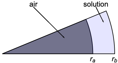
This mass transport model describes the sedimentation and diffusion of a solute under ultracentrifugation in a disk sector cell. The governing equation for describing this phenomenon is called the Lamm equation, which can be modeled with a 1D axisymmetric conservative mass transport equation:
Set up the mass transport model variable vars:
vars = {c[t, r], t, {r}};Set up a line region ![]() where
where ![]() denotes the radial position of the air-solution meniscus, which is formed during the centrifugation process, and
denotes the radial position of the air-solution meniscus, which is formed during the centrifugation process, and ![]() the radial position of the cell bottom:
the radial position of the cell bottom:
Subscript[r, a] = 5.8;
Subscript[r, b] = 7.2;
Ω = Line[{{Subscript[r, a]}, {Subscript[r, b]}}];
Specify the model parameter's species diffusivity ![]() in
in ![]() and fluid flow velocity
and fluid flow velocity ![]() , where
, where ![]() is the sedimentation coefficient in seconds (
is the sedimentation coefficient in seconds (![]() ) and
) and ![]() the angular velocity in
the angular velocity in ![]() :
:
pars = <|"DiffusionCoefficient" -> {d}, "RegionSymmetry" -> "Axisymmetric", "MassConvectionVelocity" -> {sc ω ^ 2 r}, "ModelForm" -> "Conservative"|>;Set up the parameters with an initial unity concentration:
parameters = {c0 -> 1, sc -> 1.562*^-12, ω -> 5236, d -> 1.279*^-7};Set up the initial conditions:
ic = {c[0, r] == c0};The flux is zero at both boundaries of the domain, so the boundary condition used is the MassImpermeableBoundaryValue that is applied at ![]() .This specific boundary is the implicit default boundary condition for the conservative model.
.This specific boundary is the implicit default boundary condition for the conservative model.
pde = {MassTransportPDEComponent[vars, pars] == 0, ic} /. parameters;Cfun = NDSolveValue[pde, c, {t, 0, 2525}, r∈ NDSolve`FEM`ToGradedMesh[Ω, <|"Alignment" -> "Right", "ElementCount" -> 700|>]]Visualize the concentrations at various points in time:
Plot[{Cfun[0, r], Cfun[101, r], Cfun[404, r], Cfun[1010, r], Cfun[2525, r]}, {r, Subscript[r, a], Subscript[r, b]}, PlotRange -> {0, 1.5}, AxesLabel -> {r, "C"}, PlotLegends -> {"t=0 s", "t=101 s", "t=404 s", "t=1010 s", "t=2525 s"}]Model mass transport of a pollutant in a 2D rectangular region in an isotropic homogeneous medium. Initially, the pollutant concentration is zero throughout the region of interest. A concentration of 3000 ![]() is maintained at a strip with dimension 0.2
is maintained at a strip with dimension 0.2 ![]() located at the center of the left boundary, while a pollutant outflow of 100
located at the center of the left boundary, while a pollutant outflow of 100 ![]() is applied at both the top and bottom boundaries. A diffusion coefficient of 0.833
is applied at both the top and bottom boundaries. A diffusion coefficient of 0.833 ![]() is distributed uniformly, but both horizontal and vertical velocity are spatial dependent:
is distributed uniformly, but both horizontal and vertical velocity are spatial dependent:
Set up the mass transport model variables vars:
vars = {c[x, y], {x, y}};Set up a rectangular domain with a width of ![]() and a height of
and a height of ![]() :
:
Ω = Rectangle[{0, 0}, {20, 10}];Specify the model parameters species diffusivity ![]() and fluid flow velocity
and fluid flow velocity ![]() :
:
pars = <|"DiffusionCoefficient" -> 0.833, "MassConvectionVelocity" -> {0.01x ^ 2, -0.02y}|>;Set up a species concentration source of 0.2 ![]() length at the center of the left surface:
length at the center of the left surface:
Subscript[Γ, C] = MassConcentrationCondition[x == 0 && 4.9 ≤ y ≤ 5.1, vars, pars, <|"MassConcentration" -> 3000|>]Set up an outflow flux ![]() of
of ![]() on the top and bottom surfaces:
on the top and bottom surfaces:
Subscript[Γ, flux] = MassFluxValue[y == 0 || y == 10, vars, pars, <|"MassFlux" -> -10|>]eqn = {MassTransportPDEComponent[vars, pars] == Subscript[Γ, flux], Subscript[Γ, C]}cfun = NDSolveValue[eqn, c, {x, y}∈Ω];ContourPlot[cfun[x, y], {x, y}∈Ω, Rule[...]]Set up a Fokker–Planck equation:
Set up the mass transport model variables vars:
vars = {c[t, x, y], t, {x, y}};Ω = Rectangle[{-10, -10}, {10, 10}];Specify the model parameters species diffusivity ![]() , the convection velocity term and parameters:
, the convection velocity term and parameters:
pars = <|"ModelForm" -> "Conservative", "DiffusionCoefficient" -> {{0, 0}, {0, d}}, "MassConvectionVelocity" -> {y, -2ξ ω y - x}, d -> 1 / 10, ω -> 1, ξ -> 1 / 20, μ -> {5, 5}, σ -> 1 / 9 * IdentityMatrix[2]|>;ics = c[0, x, y] == PDF[MultinormalDistribution[μ, σ] /. pars, {x, y}]eqn = {MassTransportPDEComponent[vars, pars] == 0, ics}In this case, a first-order mesh is sufficient to solve the Fokker–Planck equation. Using a higher mesh order will result in an increased memory consumption. While solving, NDSolve will warn about the convection-dominant nature of the PDE:
cfun = Monitor[NDSolveValue[eqn, c, {t, 0, 100}, {x, y}∈Ω, Method -> {"PDEDiscretization" -> {"MethodOfLines", {"SpatialDiscretization" -> {"FiniteElement", "MeshOptions" -> {"MaxCellMeasure" -> 0.05, "MeshOrder" -> 1}}}}}, EvaluationMonitor :> (monitor = Row[{"t = ", CForm[t]}])], monitor]Visualize the expected solution at the point {0,0}:
Plot[cfun[t, 0, 0], {t, 0, 100}, Ticks -> {Automatic, Range[0, 0.18, 0.02]}, GridLines -> {Automatic, Range[0, 0.18, 0.02]}]The Smoluchowski diffusion equation is a special case of the Fokker–Plank equation. Both equations can be modeled with a conservative mass transport equation:
Set up the mass transport model variables vars:
vars = {c[t, x], t, {x}};Set up a line domain with a width of 8 units:
Ω = Line[{{-8}, {8}}];Specify the model parameters species diffusivity ![]() and a migration term that depends on a linear potential U(x) that relates to F(x) with F(x)=-∇xU(x):
and a migration term that depends on a linear potential U(x) that relates to F(x) with F(x)=-∇xU(x):
U[x_] := γ * x
pars = <|"ModelForm" -> "Conservative", "DiffusionCoefficient" -> {{d}}, "MassConvectionVelocity" -> β  * (-Grad[U[x], {x}]), d -> 1, γ -> 1, β -> 1|>;
Set up the known analytical solution:
solution[t_, x_] := Evaluate[With[{x0 = 0, t0 = 0},
	1 / Sqrt[4 π d (t - t0)] * Exp[-(x - x0 + d β γ (t - t0)) ^ 2 / (4d  * (t - t0))]] /. pars]
Set up the initial conditions at ![]() from the analytical solution:
from the analytical solution:
ics = c[1 / 10, x] == solution[1 / 10, x];eqn = {MassTransportPDEComponent[vars, pars] == 0, ics}cfun = NDSolveValue[eqn, c, {t, 1 / 10, 1}, {x}∈Ω];frames = Table[Plot[cfun[t, x], {x}∈Ω, PlotRange -> {0, 1}], {t, 1 / 10, 1, 1 / 10}];
ListAnimate[frames, SaveDefinitions -> True]Plot[{solution[1, x] - cfun[1, x]}, {x}∈Ω, PlotRange -> All]Coupled Equations (3)
Solve a coupled heat and mass transport model:
)/(partialt)+del .(-k del Theta(t,x))-Q^(︷^( heat transfer model )) = 0; (partialc(t,x))/(partialt)+del .(-d del c(t,x))-R^(︷^( mass transport model )) = 0")
Set up the heat transfer mass transport model variables vars:
hvars = {Θ[t, x], t, {x}};
mvars = {c[t, x], t, {x}};Ω = Line[{{0}, {1}}];Specify heat transfer and mass transport model parameters, heat source ![]() , thermal conductivity
, thermal conductivity ![]() , mass diffusivity
, mass diffusivity ![]() and mass source
and mass source ![]() :
:
pars = <|"ThermalConductivity" -> 0.01, "HeatSource" -> 0.2 * R, "DiffusionCoefficient" -> 0.01, "MassSource" -> R, R -> -10 ^ -3 * Θ[t, x] * c[t, x]|>;Set up the model and initial conditions:
eqn = {HeatTransferPDEComponent[hvars, pars] == 0, MassTransportPDEComponent[mvars, pars] == 0}ics = {Θ[0, x] == 200 + 800x, c[0, x] == 800};{Tfun, cfun} = NDSolveValue[{eqn, ics}, {Θ, c}, {t, 0, 10}, {x}∈Ω];Manipulate[Plot[{cfun[t, x], Tfun[t, x]}, {x}∈Ω, ...], {{t, 1.3}, 0, 10}, Rule[...]]Solve a coupled heat transfer and mass transport model with a thermal transfer value and a mass flux value on the boundary:
)/(partialt)+del .(-k del Theta(t,x))-Q^(︷^( heat transfer model )) = |_(Gamma_(x=1))h (Theta_(ext)(t,x)-Theta(t,x))^(︷^( heat transfer boundary )); (partialc(t,x))/(partialt)+del .(-d del c(t,x))-R^(︷^( mass transport model )) = |_(Gamma_(x=0||x=1))q (t,x)^(︷^( mass flux boundary ))")
Set up the heat transfer mass transport model variables vars:
hvars = {Θ[t, x], t, {x}};
mvars = {c[t, x], t, {x}};Ω = Line[{{0}, {1}}];Specify heat transfer and mass transport model parameters, heat source ![]() , thermal conductivity
, thermal conductivity ![]() , mass diffusivity
, mass diffusivity ![]() and mass source
and mass source ![]() :
:
pars = <|"ThermalConductivity" -> 0.01, "HeatSource" -> 0.2 * R, "DiffusionCoefficient" -> 0.01, "MassSource" -> R, R -> -10 ^ -3 * Θ[t, x] * c[t, x]|>;Specify boundary condition parameters for a thermal convection value with an external flow temperature ![]() of 1000 K and a heat transfer coefficient
of 1000 K and a heat transfer coefficient ![]() of
of ![]() :
:
pars["BC1"] = <|"AmbientTemperature" -> 1000, "HeatTransferCoefficient" -> 0.1|>;eqn = {HeatTransferPDEComponent[hvars, pars] == HeatTransferValue[x == 1, hvars, pars, "BC1"], MassTransportPDEComponent[mvars, pars] == NeumannValue[20, x == 0 || x == 1]}ics = {Θ[0, x] == 200 + 800x, c[0, x] == 800};{Tfun, cfun} = NDSolveValue[{eqn, ics}, {Θ, c}, {t, 0, 10}, {x, 0, 1}];Manipulate[Plot[{cfun[t, x], Tfun[t, x]}, {x}∈Ω, ...], {{t, 1.7}, 0, 10}, Rule[...]]A numeric cyclic voltammetry can be performed by solving a coupled reaction model:
)/(partialt)+del .(-d_A del c_A(t,x))^(︷^( mass transport model )) = |_(Gamma_(x=0))k_cc_A (t,x)-k_ac_B(t,x)^(︷^( mass transfer boundary )); (partialc_B(t,x))/(partialt)+del .(-d_B del c_B(t,x))^(︷^( mass transport model )) = |_(Gamma_(x=0))k_ac_B (t,x)-k_cc_A(t,x)^(︷^( mass transfer boundary ))")
The underlying reaction model is given by
Set up the mass transport model variables vars:
vars = {{cA[t, x], cB[t, x]}, t, {x}};Ω = Line[{{0}, {1 / 40}}];cAbulk = 1;
dA = 10 ^ -5;dB = 10 ^ -5;Specify the electrochemical rate constants:
k0 = 10 ^ -5;α = 1 / 2;β = 1 / 2;ef0 = 0;rtbyf = 25.7 10 ^ -3;
kc[t_] := Evaluate[k0 Exp[-α / rtbyf (e[t] - ef0)]]
ka[t_] := Evaluate[k0 Exp[β / rtbyf (e[t] - ef0)]]ts = 1;ν = -1;e1 = 1 / 2;
e[t_] := Evaluate[Piecewise[{{e1 + ν t, 0 ≤ t ≤ ts}, {e1 + 2 ν ts - ν t, ts ≤ t ≤ 2 ts}}]]Specify mass transport model parameters, mass diffusivity ![]() and
and ![]() . The concentration of
. The concentration of ![]() at the far end is set to the bulk concentration and the concentration of
at the far end is set to the bulk concentration and the concentration of ![]() is set to 0:
is set to 0:
pars = <|"DiffusionCoefficient" -> {{dA, 0}, {0, dB}}, "BoundaryCondition1" -> <|"AmbientConcentration" -> {ka[t] / kc[t] cB[t, x], kc[t] / ka[t] cA[t, x]}, "MassTransferCoefficient" -> {kc[t], ka[t]}|>, "BoundaryCondition2" -> <|"MassConcentration" -> {cAbulk, 0}|>|>;eqn = {MassTransportPDEComponent[vars, pars] == MassTransferValue[x == 0, vars, pars, "BoundaryCondition1"], MassConcentrationCondition[x == 1 / 40, vars, pars, "BoundaryCondition2"]};Set up initial conditions such that only ![]() is in bulk solution:
is in bulk solution:
ics = {cA[0, x] == cAbulk, cB[0, x] == 0};tmax = 2 ts;
{cAfun, cBfun} = NDSolveValue[{eqn, ics}, {cA, cB}, {t, 0, tmax}, {x}∈Ω];Visualize the concentrations at various points in time:
Manipulate[Plot[{cAfun[t, x], cBfun[t, x]}, {x, 0, 1 / 20}, ...], {...}, Rule[...]]Visualize the cyclic voltammogram at various points in time:
Manipulate[ParametricPlot[{-(e[t] - ef0), kc[t] (cAfun[t, 0] - (ka[t] cBfun[t, 0]) / kc[t])}, {t, 0, tmax}, ...], {...}, Rule[...]]Properties & Relations (1)
Model a 1D chemical species field once with a conservative model and once with a non-conservative model. For a constant velocity flow field, both models return the same result. The right side and left side are subjected to a mass concentration and inflow conditions, respectively:
Set up the stationary mass transport model variables vars:
vars = {c[x], {x}};Ω = Line[{{0}, {1}}];Specify the mass transport model parameters species diffusivity ![]() and fluid flow velocity
and fluid flow velocity ![]() :
:
pars1 = <|"DiffusionCoefficient" -> 0.026, "MassConvectionVelocity" -> {0.1}|>;
pars2 = Join[pars1, <|"ModelForm" -> "Conservative"|>];
Specify mass concentration boundary condition:
massConditons1 = MassConcentrationCondition[x == 1, vars, pars1, <|"MassConcentration" -> 0|>];massConditons2 = MassConcentrationCondition[x == 1, vars, pars2, <|"MassConcentration" -> 0|>];Specify species flux boundary condition:
Subscript[Γ, flux1] = MassFluxValue[x == 0, vars, pars1, <|"MassFlux" -> 1|>];
Subscript[Γ, flux2] = MassFluxValue[x == 0, vars, pars2, <|"MassFlux" -> 1|>];eqn1 = MassTransportPDEComponent[vars, pars1] == Subscript[Γ, flux1];
eqn2 = MassTransportPDEComponent[vars, pars2] == Subscript[Γ, flux2];cfun1 = NDSolveValue[{eqn1, massConditons1}, c, x∈Ω]cfun2 = NDSolveValue[{eqn2, massConditons2}, c, x∈Ω]Visualize that the difference in the solutions is minimal:
Plot[{cfun1[x] - cfun2[x]}, x∈Ω, AxesLabel -> {"x", "c"}, PlotLegends -> "Expressions"]Possible Issues (2)
The implicit default boundary condition changes depending on the model form. For a conservative model, an implicit Neumann 0 boundary condition is equivalent to specifying an impermeable boundary condition. For a non-conservative model, an implicit Neumann 0 boundary condition is equivalent to specifying an outflow boundary condition.
Considering this, for a constant velocity field, both the conservative and non-conservative models return the same result. A comparison between the conservative and non-conservative fields are conducted based on the following models:
Set up the mass transport model variables vars:
vars = {c[x, y], {x, y}};Ω = Rectangle[{0, 0}, {2, 1}];Specify the model parameters species diffusivity ![]() and fluid flow velocity
and fluid flow velocity ![]() :
:
pars1 = <|"DiffusionCoefficient" -> 1, "MassConvectionVelocity" -> {0.01, -0.02}|>;
pars2 = Join[pars1, <|"ModelForm" -> "Conservative"|>];
Set up a species concentration source of 0.2 ![]() length at the center of the left surface:
length at the center of the left surface:
Subscript[Γ, concentration1] = MassConcentrationCondition[x == 0 && 0.4 ≤ y ≤ 0.6, vars, pars1, <|"MassConcentration" -> 1|>]Subscript[Γ, concentration2] = MassConcentrationCondition[x == 0 && 0.4 ≤ y ≤ 0.6, vars, pars2, <|"MassConcentration" -> 1|>]Set up an outflow flux ![]() of
of ![]() on the top and bottom surfaces:
on the top and bottom surfaces:
Subscript[Γ, flux1] = MassFluxValue[y == 0 || y == 10, vars, pars1, <|"MassFlux" -> -1|>]Subscript[Γ, flux2] = MassFluxValue[y == 0 || y == 10, vars, pars2, <|"MassFlux" -> -1|>]Since the default boundary condition for a conservative model is an impermeable boundary, an impermeable boundary condition is added to the non-conservative mode:
Subscript[Γ, imp] = MassImpermeableBoundaryValue[(x == 0 && (y < 4.9 || y > 5.1)) || x == 20, vars, pars1]eqn1 = {MassTransportPDEComponent[vars, pars1] == Subscript[Γ, flux1] + Subscript[Γ, imp], Subscript[Γ, concentration1]};
eqn2 = {MassTransportPDEComponent[vars, pars2] == Subscript[Γ, flux2], Subscript[Γ, concentration2]};cfun1 = NDSolveValue[eqn1, c, {x, y}∈Ω];
cfun2 = NDSolveValue[eqn2, c, {x, y}∈Ω];Visualize the difference in the solutions:
ContourPlot[cfun1[x, y] - cfun2[x, y], {x, y}∈Ω, PlotLegends -> Automatic]The scale of the differences in the solutions is expected and comes from numerical differences in how the operators are computed.
When a discretized region is given and the mesh does not meet the quality criteria for a large convection-to-diffusion ratio, a message is generated. Model a 1D non-conservative chemical species field with a high convection velocity to diffusivity ratio, expressed as follows:
Set up the mass transport model variables vars:
vars = {c[t, x], t, {x}};Ω = Line[{{0}, {1}}];Specify a nonlinear species diffusivity ![]() and fluid flow velocity
and fluid flow velocity ![]() :
:
pars = <|"DiffusionCoefficient" -> 0.005, "MassConvectionVelocity" -> {1}|>;Specify an outflow flux ![]() of
of ![]() applied at the right end:
applied at the right end:
Subscript[Γ, flux] = MassFluxValue[x == 1, vars, pars, <|"MassFlux" -> -1|>]Specify mass concentration surface conditions:
massConditons = MassConcentrationCondition[x == 0, vars, pars, <|"MassConcentration" -> 100 + 0.1 * t|>];ics = c[0, x] == 100;eqn = MassTransportPDEComponent[vars, pars] == Subscript[Γ, flux]cfun = NDSolveValue[{eqn, ics, massConditons}, c, {t, 0, 500}, x∈NDSolve`FEM`ToElementMesh[Ω]];Solve the PDE with a refined mesh:
cfun = NDSolveValue[{eqn, ics, massConditons}, c, {t, 0, 500}, x∈NDSolve`FEM`ToElementMesh[Ω, "MaxCellMeasure" -> 0.01]]Text
Wolfram Research (2020), MassTransportPDEComponent, Wolfram Language function, https://reference.wolfram.com/language/ref/MassTransportPDEComponent.html (updated 2021).
CMS
Wolfram Language. 2020. "MassTransportPDEComponent." Wolfram Language & System Documentation Center. Wolfram Research. Last Modified 2021. https://reference.wolfram.com/language/ref/MassTransportPDEComponent.html.
APA
Wolfram Language. (2020). MassTransportPDEComponent. Wolfram Language & System Documentation Center. Retrieved from https://reference.wolfram.com/language/ref/MassTransportPDEComponent.html