

范例
打开所有单元 关闭所有单元基本范例 (4)
PDF[NormalDistribution[0, 1], x]Plot[%, {x, -5, 5}, Filling -> Axis]PDF[HypergeometricDistribution[20, 50, 100], k]DiscretePlot[%, {k, 0, 20}, ExtentSize -> 0.5]PDF[BinormalDistribution[1 / 3], {x, y}]Plot3D[%, {x, -3, 3}, {y, -3, 3}]PDF[MultivariatePoissonDistribution[1, {2, 3}], {x, y}]DiscretePlot3D[%, {x, 0, 10}, {y, 0, 10}, ExtentSize -> 0.5]范围 (25)
参数分布 (7)
PDF[WeibullDistribution[2, 5], 4]PDF[NegativeBinomialDistribution[20, 1 / 3], 5]PDF[WeibullDistribution[2, 5], 4.]PDF[WeibullDistribution[2, 5], N[4, 25]]PDF[NegativeBinomialDistribution[20, N[1 / 3, 30]], 5]获取 PDF 的符号表达式:
PDF[ChiSquareDistribution[ν], x]PDF[UniformDistribution[{{a, b}, {c, d}}], {x, y}]PDF[GammaDistribution[1, 2]]%[3]PDF 线性作用于列表:
PDF[NormalDistribution[], {0.0, 0.2, 0.3}]PDF[BinormalDistribution[1 / 2], {{0.0, 0.0}, {0.2, 0.2}, {0.3, 0.3}}]非参数分布 (4)
分参数分布的 PDF:
r = RandomVariate[NormalDistribution[], 10 ^ 4];PDF[HistogramDistribution[r], 0.2]PDF[SmoothKernelDistribution[r], 0.2]PDF[NormalDistribution[], 0.2]Plot[PDF[HistogramDistribution[RandomVariate[NormalDistribution[], 10 ^ 3]], x]//Evaluate, {x, -3, 3}, Filling -> Axis]PDF[KernelMixtureDistribution[RandomVariate[GammaDistribution[1, 2], 10
]], x]Plot3D[PDF[SmoothKernelDistribution[RandomVariate[BinormalDistribution[1 / 3], 30]], {x, y}]//Evaluate, {x, -3, 3}, {y, -3, 3}, PlotRange -> {0, 0.4}]导出分布 (10)
pdf = PDF[ProductDistribution[TriangularDistribution[{2, 4}], TriangularDistribution[{1, 7}]], {x, y}]Plot3D[pdf, {x, 1, 5}, {y, 0, 8}, PlotRange -> All]pdf = PDF[MixtureDistribution[{1, 4}, {NormalDistribution[a, b], NormalDistribution[c, d]}], x]Plot[pdf /. {a -> 0, b -> 1, c -> 6, d -> 3 / 2}, {x, -2, 10}, Filling -> Axis]PDF[TransformedDistribution[x ^ 2, xPoissonDistribution[2]], y]DiscretePlot[%, {y, 0, 50}, PlotRange -> {0, 0.3}]PDF[CensoredDistribution[{-2, 4}, CauchyDistribution[0, 1]], x]Integrate[%, {x, -Infinity, Infinity}]PDF[TruncatedDistribution[{2, 3}, TriangularDistribution[{1, 4}]], x]Plot[{PDF[TriangularDistribution[{1, 4}], x], %}, {x, 1, 5}, Filling -> Axis]PDF[ParameterMixtureDistribution[PoissonDistribution[μ], μUniformDistribution[{2, 3}]], x]PDF[CopulaDistribution[{"Frank", 3}, {ExponentialDistribution[2], ExponentialDistribution[5]}], {x, y}]NIntegrate[%, {x, -Infinity, Infinity}, {y, -Infinity, Infinity}]PDF[ProbabilityDistribution[(Sqrt[2] / Pi)(1 / (1 + x ^ 4)), {x, -Infinity, Infinity}], x]PDF[ProbabilityDistribution[{"CDF", Piecewise[{{-2 + x, 2 ≤ x ≤ 3}, {1, x > 3}}, 0]}, {x, -Infinity, Infinity}], x]PDF[ProbabilityDistribution[{"SF", Piecewise[{{1 - 2(-2 + x) ^ 2, 2 ≤ x ≤ 5 / 2}, {2(3 - x) ^ 2, 5 / 2 < x ≤ 3}, {1, x < 2}}, 0]}, {x, -Infinity, Infinity}], x]PDF[MarginalDistribution[
ProbabilityDistribution[1 / (E ^ (y ^ 2 / 2)(Pi ^ (3 / 2)(1 + x ^ 4))),
{x, -Infinity, Infinity}, {y, -Infinity, Infinity}], 2], y]QuantityDistribution 的概率密度函数假定参数为具有兼容单位的 Quantity:
𝒟 = NormalDistribution[Quantity[4, "Meters"], Quantity[1 / 2, "Meters"]]PDF[𝒟, x]% /. x -> Quantity[387., "Centimeters"]PDF[𝒟, Quantity[387., "Centimeters"]]随机过程 (4)
求离散状态随机过程的 SliceDistribution 的概率密度函数:
PDF[PoissonProcess[μ][2], x]DiscretePlot[Evaluate[% /. μ -> 2], {x, 0, 15}, ExtentSize -> 0.5]PDF[WienerProcess[][2], x]Plot[%, {x, -3, 3}, Filling -> Axis]PDF[PoissonProcess[μ][{2, 3}], {x, y}]DiscretePlot3D[Evaluate[% /. μ -> 2], {x, 0, 10}, {y, 0, 10}, ExtentSize -> 0.5]PDF[WienerProcess[][{2, 3}], {x, y}]Plot3D[%, {x, -3, 3}, {y, -3, 3}]求离散状态随机过程的 StationaryDistribution 的概率密度函数:
PDF[StationaryDistribution[QueueingProcess[λ, μ, 2]], x]//FullSimplifyDiscretePlot[Evaluate[% /. {μ -> 3, λ -> 2.9}], {x, 0, 10}, ExtentSize -> 0.5]
PDF[WienerProcess[1, 1][t], x]Plot3D[%, {x, -3, 8}, {t, 1, 5}, AxesLabel -> Automatic, PlotRange -> All]应用 (10)
绘制概率密度函数 (5)
Plot[PDF[NormalDistribution[0, 1], x], {x, -3, 3}]DiscretePlot[PDF[PoissonDistribution[10], x], {x, 0, 30}]Plot3D[PDF[DirichletDistribution[{3, 2, 5}], {x, y}], {x, 0, 1}, {y, 0, 1}, AxesLabel -> Automatic, PlotRange -> All, Exclusions -> None]DiscretePlot3D[PDF[MultivariatePoissonDistribution[1, {2, 3}], {x, y}], {x, 0, 10}, {y, 0, 10}, PlotRange -> All]DiscretePlot3D[PDF[MultivariatePoissonDistribution[1, {2, 3}], {x, y}], {x, 0, 10}, {y, 0, 10}, PlotRange -> All, ExtentSize -> Full, PlotStyle -> Lighter[Blue, 0.5]]Plot3D[PDF[NormalDistribution[0, σ], x], {σ, 1 / 2, 2}, {x, -3, 3}, AxesLabel -> Automatic]计算累积分布函数 (1)
置信区间 (1)
pdf = PDF[NormalDistribution[], x]{xl, xr} = Function[α, Quantile[NormalDistribution[], {(1 - α/2.0), (1 + α/2.0)}]][Quantity[70, "Percent"]]Show[Plot[pdf, {x, -1.7, 1.7}, Filling -> Axis, AxesOrigin -> {0, 0}, RegionFunction -> (Not[xl < # < xr]&)], Plot[pdf, {x, xl, xr}], PlotRange -> {0, 0.4}, Ticks -> {Automatic, None}]分布模式 (1)
仿射变换 (1)


属性和关系 (9)
Integrate[PDF[GammaDistribution[α, β], x], {x, 0, Infinity}, Assumptions -> α > 0 && β > 0]Sum[PDF[GeometricDistribution[p], k], {k, 0, Infinity}]


Integrate[PDF[ExponentialDistribution[λ], ξ], {ξ, -∞, x}, Assumptions -> x∈Reals && λ > 0]CDF[ExponentialDistribution[λ], x]FullSimplify[%% - %, λ > 0]


𝒟 = DirichletDistribution[{1, 2, 3}];int = Integrate[PDF[𝒟, {ξ, ψ}], {ξ, -∞, x}, {ψ, -∞, y}, Assumptions -> {x, y}∈Reals];cdf = CDF[𝒟, {x, y}];FullSimplify[int - cdf, {x, y}∈Reals]


Sum[PDF[GeometricDistribution[p], m], {m, -∞, Floor[n]}]//FullSimplifyCDF[GeometricDistribution[p], n]FullSimplify[% - %%, Im[n] == 0]


Integrate[PDF[ExponentialDistribution[λ], ξ], {ξ, x, ∞}, Assumptions -> x∈Reals && λ > 0]SurvivalFunction[ExponentialDistribution[λ], x]FullSimplify[%% - %, λ > 0]连续分布  的 Expectation 是一个以概率密度函数为权数的积分
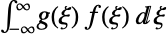 :
𝒟 = ChiSquareDistribution[ν];Simplify[Subsuperscript[∫, 0, ∞]x^2 PDF[𝒟, x]ⅆx, ν > 0]Expectation[x^2, x𝒟]

𝒟 = PoissonDistribution[μ];Subsuperscript[∑, ξ = 0, ∞]ξ^2PDF[𝒟, ξ]Expectation[ξ ^ 2, ξ𝒟]
Probability[x == 5, xPoissonDistribution[m]]PDF[PoissonDistribution[m], 5]分布的 HazardFunction 是概率密度函数与生存函数之比:
HazardFunction[NormalDistribution[], x]PDF[NormalDistribution[], x] / SurvivalFunction[NormalDistribution[], x]可能存在的问题 (3)
对于某些分布,不存在相应的符号式解析表达式(closed form):
PDF[StableDistribution[0, 1.8, -0.5, 1, 2], x]PDF[StableDistribution[0, 1.8, -0.5, 1, 2], 0.3]PDF[CauchyDistribution[2, 3], x] /. {x -> I}PDF[CauchyDistribution[2, 3], I]度量与 Lebesgue 度量或整数点阵上的计数度量不兼容的分布的 PDF 可能不计算或给出不正确的结果:
𝒟 = TransformedDistribution[x y, {xUniformDistribution[{0, 1}], yDiscreteUniformDistribution[{0, 1}]}];PDF 的结果没有归一化:
PDF[𝒟, x]分布度量在原点有原子,因此不与 Lebesgue 度量兼容:
Probability[x == 0, x𝒟]不兼容性表现在原子位置的 CDF 的跳跃不连续性:
cdf = CDF[𝒟, x]Plot[cdf, {x, -0.1, 1}, ExclusionsStyle -> {Directive[Thick, Red], Directive[PointSize[Large], Red]}, Filling -> Axis]Expectation、Probability、RandomVariate 等完全支持混合分布:
Expectation[Log[1 + x], x𝒟]Log[1 + RandomVariate[𝒟, 10 ^ 5]]//Mean巧妙范例 (3)
𝒟 = TruncatedDistribution[{{-∞, 1 / 2}, {-∞, ∞}}, BinormalDistribution[1 / 7]];Plot3D[{PDF[𝒟 , {x, y}], PDF[BinormalDistribution[(1/7)], {x, y}]}//Evaluate, {x, -3, 3}, {y, -3, 3}, PlotRange -> All, PlotPoints -> 35]Σ = With[{σ1 = 1, σ2 = 2, σ3 = 1, ρ23 = 0, ρ13 = 0}, {{σ1 ^ 2, σ1 σ2 ρ12, σ1 σ3 ρ13}, {σ1 σ2 ρ12, σ2 ^ 2, σ2 σ3 ρ23}, {σ1 σ3 ρ13, σ2 σ3 ρ23, σ3 ^ 2}}];
μ = {0., 0, 0};Block[{ρ12 = 1 / 2}, ContourPlot3D[PDF[MultinormalDistribution[μ, Σ], {x, y, z}]//Evaluate, {x, -3, 3}, {y, -3, 3}, {z, -3, 3}, Mesh -> None, Contours -> 4, ContourStyle -> {Red, Yellow, Green, Blue}, RegionFunction -> Function[{x, y, z}, x < 0 || y > 0], PlotLabel -> ρ12, PlotRange -> Full]]Σ = With[{σ1 = 1, σ2 = 2, σ3 = 1, ρ23 = 0, ρ13 = 0}, {{σ1 ^ 2, σ1 σ2 ρ12, σ1 σ3 ρ13}, {σ1 σ2 ρ12, σ2 ^ 2, σ2 σ3 ρ23}, {σ1 σ3 ρ13, σ2 σ3 ρ23, σ3 ^ 2}}];
μ = {0., 0, 0};
DistributeDefinitions[μ, Σ];ParallelTable[
ContourPlot3D[PDF[MultinormalDistribution[μ, Σ], {x, y, z}]//Evaluate, {x, -3, 3}, {y, -3, 3}, {z, -3, 3}, Mesh -> None, Contours -> {0.01}, PlotLabel -> ρ12, PlotRange -> Full], {ρ12, {-0.95, -0.75, -0.5, -0.25, 0, 0.25, 0.5, 0.75, 0.95}}]
 《Wolfram 语言入门》:创建网站和应用程序
文本
Wolfram Research (2007),PDF,Wolfram 语言函数,https://reference.wolfram.com/language/ref/PDF.html (更新于 2010 年).
CMS
Wolfram 语言. 2007. "PDF." Wolfram 语言与系统参考资料中心. Wolfram Research. 最新版本 2010. https://reference.wolfram.com/language/ref/PDF.html.
APA
Wolfram 语言. (2007). PDF. Wolfram 语言与系统参考资料中心. 追溯自 https://reference.wolfram.com/language/ref/PDF.html 年