

ParallelTable
ParallelTable[expr,{imax}]
generates in parallel a list of imax copies of expr.
ParallelTable[expr,{i,imax}]
generates in parallel a list of the values of expr when i runs from 1 to imax.
ParallelTable[expr,{i,imin,imax}]
starts with i=imin.
ParallelTable[expr,{i,imin,imax,di}]
uses steps di.
ParallelTable[expr,{i,{i1,i2,…}}]
uses the successive values i1, i2, ….
ParallelTable[expr,{i,imin,imax},{j,jmin,jmax},…]
gives a nested list. The list associated with i is outermost.
Details and Options
- ParallelTable is a parallel version of Table that automatically distributes different evaluations of expr among different kernels and processors.
- ParallelTable will give the same results as Table, except for side effects during the computation.
- Parallelize[Table[expr,iter, …]] is equivalent to ParallelTable[expr,iter,…].
- If an instance of ParallelTable cannot be parallelized, it is evaluated using Table.
- The following options can be given:
-
Method Automatic granularity of parallelization DistributedContexts $DistributedContexts contexts used to distribute symbols to parallel computations ProgressReporting $ProgressReporting whether to report the progress of the computation - The Method option specifies the parallelization method to use. Possible settings include:
-
"CoarsestGrained" break the computation into as many pieces as there are available kernels "FinestGrained" break the computation into the smallest possible subunits "EvaluationsPerKernel"->e break the computation into at most e pieces per kernel "ItemsPerEvaluation"->m break the computation into evaluations of at most m subunits each Automatic compromise between overhead and load balancing - Method->"CoarsestGrained" is suitable for computations involving many subunits, all of which take the same amount of time. It minimizes overhead, but does not provide any load balancing.
- Method->"FinestGrained" is suitable for computations involving few subunits whose evaluations take different amounts of time. It leads to higher overhead, but maximizes load balancing.
- By default, a nested table with a large outermost level is parallelized at the outermost level, otherwise, at the innermost level. With Method->"CoarsestGrained", it is parallelized at the outermost level. With Method->"FinestGrained", it is parallelized at the innermost level.
- The DistributedContexts option specifies which symbols appearing in expr have their definitions automatically distributed to all available kernels before the computation.
- The default value is DistributedContexts:>$DistributedContexts with $DistributedContexts:=$Context, which distributes definitions of all symbols in the current context but does not distribute definitions of symbols from packages.
- The ProgressReporting option specifies whether to report the progress of the parallel computation.
- The default value is ProgressReporting:>$ProgressReporting.
Examples
open all close allBasic Examples (6)
ParallelTable works like Table, but in parallel:
Table[Pause[1];f[i], {i, 4}]//AbsoluteTimingParallelTable[Pause[1];f[i], {i, 4}]//AbsoluteTimingA table of the first 10 squares:
ParallelTable[i ^ 2, {i, 10}]A table with i running from 0 to 20 in steps of 2:
ParallelTable[f[i], {i, 0, 20, 2}]ParallelTable[10i + j, {i, 4}, {j, 3}]MatrixForm[%]ListPlot[ParallelTable[Total[FactorInteger[2 ^ i - 1][[All, 2]]], {i, 150, 190}]]Longer computations display information about their progress and estimated time to completion:
res = ParallelTable[PrimeQ[2 ^ i - 1], {i, 9601, 12000}];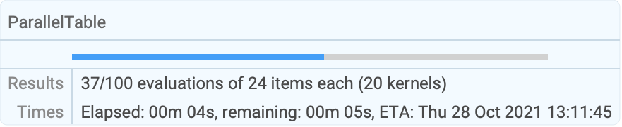
| |
Scope (5)
The index in the table can run backward:
ParallelTable[f[i], {i, 10, -5, -2}]ParallelTable[10i + j, {i, 5}, {j, i}]TableForm[%]Make a 3x2x4 array, or tensor:
ParallelTable[100i + 10j + k, {i, 3}, {j, 2}, {k, 4}]Iterate over an existing list:
ParallelTable[Sqrt[x], {x, {1, 4, 9, 16}}]Make an array from existing lists:
ParallelTable[j ^ (1 / i), {i, {1, 2, 4}}, {j, {1, 4, 9}}]Generalizations & Extensions (1)
Options (14)
Method (7)
Break the computation into the smallest possible subunits:
ParallelTable[Labeled[Framed[i], $KernelID], {i, 10}, Method -> "FinestGrained"]Break the computation into as many pieces as there are available kernels:
ParallelTable[Labeled[Framed[i], $KernelID], {i, 10}, Method -> "CoarsestGrained"]Break the computation into at most 2 evaluations per kernel for the entire job:
ParallelTable[Labeled[Framed[i], $KernelID], {i, 12}, Method -> "EvaluationsPerKernel" -> 2]Break the computation into evaluations of at most 5 elements each:
ParallelTable[Labeled[Framed[i], $KernelID], {i, 18}, Method -> "ItemsPerEvaluation" -> 5]The default option setting balances evaluation size and number of evaluations:
ParallelTable[Labeled[Framed[i], $KernelID], {i, 18}, Method -> Automatic]Calculations with vastly differing runtimes should be parallelized as finely as possible:
ParallelTable[{i, PrimeQ[2 ^ i - 1]}, {i, 4410, 4430}, Method -> "FinestGrained"]A large number of simple calculations should be distributed into as few batches as possible:
BinCounts[ParallelTable[Mod[Floor[i * Pi], 10], {i, 10000}, Method -> "CoarsestGrained"], {0, 10}]By default, a small nested table is parallelized fully at the innermost level:
ParallelTable[{i, j, Style[$KernelID, Red]}, {i, 4}, {j, i}]To parallelize only at the first level, use Method"CoarsestGrained":
ParallelTable[{i, j, Style[$KernelID, Red]}, {i, 4}, {j, i}, Method -> "CoarsestGrained"]DistributedContexts (5)
By default, definitions in the current context are distributed automatically:
remote[x_] := {$KernelID, x ^ 3}ParallelTable[remote[i], {i, 4}]Do not distribute any definitions of functions:
local[x_] := {$KernelID, x ^ 2}ParallelTable[local[i], {i, 4}, DistributedContexts -> None]Distribute definitions for all symbols in all contexts appearing in a parallel computation:
a`f[x_] := {$KernelID, x}ParallelTable[a`f[i], {i, 4}, DistributedContexts -> Automatic]Distribute only definitions in the given contexts:
b`g[x_] := {$KernelID, -x}ParallelTable[b`g[i], {i, 4}, DistributedContexts -> {"a`"}]Restore the value of the DistributedContexts option to its default:
SetOptions[ParallelTable, DistributedContexts :> $DistributedContexts]ProgressReporting (2)
Do not show a temporary progress report:
res = ParallelTable[PrimeQ[2 ^ i - 1], {i, 9601, 12000}, ProgressReporting -> False];Use Method"FinestGrained" for the most accurate progress report:
res = ParallelTable[{i, Total[FactorInteger[10 ^ 60 + i][[All, 2]]]}, {i, 1000}, Method -> "FinestGrained"];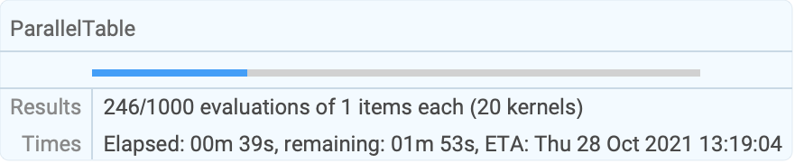
| |
Applications (5)
Solve and plot a differential equation for many initial conditions and animate the results:
eqn = D[z[t, s], t, t] == -(z[t, s]/(z[t, s]^2 + ((1/2) (1 + 0.1 Sin[2 Pi t]))^2)^3 / 2);sols = ParallelTable[localsol = NDSolve[{eqn, z[0, s] == param s, Derivative[1, 0][z][0, s] == param}, z, {t, 0, 10}, {s, 1, 2}];
Plot3D[Evaluate[z[tp, z0] /. localsol], {tp, 0, 10}, {z0, 1, 2}, PlotRange -> {-5, 5}, PlotLabel -> param],
{param, -1, 1, 0.1}];ListAnimate[sols]Explore different parameter values for the sine-Gordon equation in two spatial dimensions:
With[{L = 4, dz = 0.25},
	sols = ParallelTable[
	localsol = Quiet@NDSolve[{D[u[t, x, y], t, t] == D[u[t, x, y], x, x] + D[u[t, x, y], y, y] + Sin[u[t, x, y]], u[t, -L, y] == u[t, L, y], u[t, x, -L] == u[t, x, L], u[0, x, y] == a Exp[-(b x ^ 2 + y ^ 2)], Derivative[1, 0, 0][u][0, x, y] == 0}, u, {t, 0, L / 2}, {x, -L, L}, {y, -L, L}];
	Plot3D[Evaluate[u[L / 2, x, y] /. First[localsol]], {x, -L, L}, {y, -L, L}, PlotRange -> {{-L, L}, {-L, L}, {-dz, dz}}, Axes -> None, PlotLabel -> {a, b}], {a, -0.5, 0.5, 0.2}, {b, 0.8, 1.2, .1}, Method -> "FinestGrained"]
];GraphicsGrid[sols]Apply different algorithms to the same set of data:
img = [image];Apply a list of different filters to the same image and display the result:
filters = {Identity, Sharpen, Blur, GaussianFilter[#, 3]&, LaplacianFilter[#, 1]&, LaplacianGaussianFilter[#, 2]&,
	GradientFilter[#, 2]&, MedianFilter[#, 5]&,
ImageConvolve[#, BoxMatrix[1] / 9]&};ParallelTable[Tooltip[filter[img], filter], {filter, filters}]ParallelTable[ImageEffect[img, effect], {effect, {"Charcoal", "Embossing", "Solarization"}}]Generate 10 frames from an animation and save them to individual files:
frames[i_, f_, R_] := Module[{frame},
	Do[frame = RevolutionPlot3D[Sin[t / (10f) * 2 * Pi]BesselJ[0, r], {r, 0, R}, PlotRange -> {{-R, R}, {-R, R}, {-1, 1}}, Axes -> None, PlotPoints -> 5];
	Export["drum-" <> ToString[PaddedForm[t, 3, NumberPadding -> "0"]] <> ".gif", frame]
	, {t, 10i + 1, 10(i + 1)}
	];
	frame
	];
Run several batches in parallel:
samples = With[{batches = 8}, ParallelTable[frames[i, batches, 11], {i, 0, batches - 1}]];Each run returns one frame which can be used for checking the correctness:
samplesDeleteFile[FileNames["drum-*.gif"]]Quickly show the evaluation of several nontrivial cellular automata:
data = Select[ParallelTable[Graphics3D[{Cuboid /@ Position[CellularAutomaton[{n, {2, 1}, {1, 1, 1}}, {{{{1}}}, 0}, {{{8}}}], 1]}, Boxed -> False], {n, 2, 80, 5}], Length[#[[1, -1]]] > 50&];GraphicsGrid[Partition[data, 3], Frame -> All, ImageSize -> 500]Properties & Relations (10)
Parallelization happens along the outermost (first) index:
ParallelTable[Labeled[Framed[f[i, j]], $KernelID], {i, 4}, {j, i}]Using multiple iteration specifications is equivalent to nesting Table functions:
ParallelTable[i + j, {i, 3}, {j, i}]ParallelTable[Table[i + j, {j, i}], {i, 3}]ParallelDo evaluates the same sequence of expressions as ParallelTable:
ParallelDo[Print[i ^ i], {i, 3}]ParallelTable[i ^ i, {i, 3}]ParallelSum effectively applies Plus to results from ParallelTable:
ParallelSum[x ^ i, {i, 3}]ParallelTable[x ^ i, {i, 3}]ParallelArray iterates over successive integers:
ParallelArray[#1 ^ #2&, {3, 4}]ParallelArray[Function[{x, y}, x ^ y], {3, 4}]ParallelTable[x ^ y, {x, 3}, {y, 4}]Map applies a function to successive elements in a list:
list = RandomInteger[9, 10]ParallelMap[Last[IntegerDigits[#, 2]]&, list]Table can substitute successive elements in a list into an expression:
ParallelTable[Last[IntegerDigits[x, 2]], {x, list}]ParallelTable iterating over a given list is equivalent to ParallelCombine:
list = RandomInteger[9, 10]ParallelTable[x ^ 2, {x, list}]ParallelCombine[Function[x, x ^ 2], list]ParallelTable can be implemented with WaitAll and ParallelSubmit:
WaitAll[Table[ParallelSubmit[{i}, Labeled[Framed[f[i]], $KernelID]], {i, 4}]]Parallelization at the innermost level of a multidimensional table:
WaitAll[Table[ParallelSubmit[{i, j}, Labeled[Framed[f[i, j]], $KernelID]], {i, 4}, {j, i}]]Functions defined interactively are automatically distributed to all kernels when needed:
ftest[n_] := Labeled[Framed[PrimeQ[2 ^ n - 1]], $KernelID]ParallelTable[ftest[i], {i, 1275, 1285}]Distribute definitions manually and disable automatic distribution:
gtest[n_] := Labeled[Framed[PrimeQ[2 ^ n - 1]], $KernelID]DistributeDefinitions[gtest];ParallelTable[gtest[i], {i, 1275, 1285}, DistributedContexts -> None]For functions from a package, use ParallelNeeds rather than DistributeDefinitions:
Needs["FiniteFields`"]Table[FieldSize[GF[2, i]], {i, 10}]ParallelNeeds["FiniteFields`"]ParallelTable[FieldSize[GF[2, i]], {i, 10}]Possible Issues (3)
A function used that is not known on the parallel kernels may lead to sequential evaluation:
ftest[n_] := Labeled[Framed[PrimeQ[2 ^ n - 1]], $KernelID]ParallelTable[ftest[i], {i, 1275, 1285}, DistributedContexts -> None]Define the function on all parallel kernels:
DistributeDefinitions[ftest]The function is now evaluated on the parallel kernels:
ParallelTable[ftest[i], {i, 1275, 1285}, DistributedContexts -> None]Definitions of functions in the current context are distributed automatically:
gtest[n_] := Labeled[Framed[PrimeQ[2 ^ n - 1]], $KernelID]ParallelTable[gtest[i], {i, 1275, 1285}]Definitions from contexts other than the default context are not distributed automatically:
ctx`mtest[n_] := Labeled[Framed[PrimeQ[2 ^ n - 1]], $KernelID]ParallelTable[ctx`mtest[i], {i, 1275, 1285}]Use DistributeDefinitions to distribute such definitions:
DistributeDefinitions[ctx`mtest];ParallelTable[ctx`mtest[i], {i, 1275, 1285}]Alternatively, set the DistributedContexts option to include all contexts:
cty`mtest[n_] := Labeled[Framed[PrimeQ[2 ^ n - 1]], $KernelID]ParallelTable[cty`mtest[i], {i, 1275, 1285}, DistributedContexts -> Automatic]Trivial operations may take longer when parallelized:
AbsoluteTiming[ParallelTable[N[Sin[x]], {x, 0, 1000}];]AbsoluteTiming[Table[N[Sin[x]], {x, 0, 1000}];]Neat Examples (2)
mlength[z_] := Length[FixedPointList[# ^ 2 + z&, z, 20, SameTest -> (Abs[#] > 2&)]]points = ParallelTable[mlength[x + I y], {y, -1, 1, 0.005}, {x, -2, 1, 0.005}];ArrayPlot[points, ColorFunction -> Hue]Calculate and display the Feigenbaum (or bifurcation) diagram of the logistics map:
line[r_, dy_, np_, n0_, n_] := Module[{pts},
	With[{logistics = Function[x, r x(1 - x)]},
	pts = Join@@NestList[logistics, Nest[logistics, RandomReal[{0, 1}, np], n0], n - 1]];
Log[1.0 + BinCounts[pts, {0, 1, dy}]]]With[{w = 400, h = 250, r0 = 2.95, r1 = 4.0},
ArrayPlot[ParallelTable[line[r, 1 / (w - 1), w, 500, 50], {r, r0, r1, (r1 - r0) / (h - 1)}], ImageSize -> {w, h}]]Text
Wolfram Research (2008), ParallelTable, Wolfram Language function, https://reference.wolfram.com/language/ref/ParallelTable.html (updated 2021).
CMS
Wolfram Language. 2008. "ParallelTable." Wolfram Language & System Documentation Center. Wolfram Research. Last Modified 2021. https://reference.wolfram.com/language/ref/ParallelTable.html.
APA
Wolfram Language. (2008). ParallelTable. Wolfram Language & System Documentation Center. Retrieved from https://reference.wolfram.com/language/ref/ParallelTable.html