
PermutationMatrix
PermutationMatrix[permv]
表示由置换向量 permv 作为结构化数组给出的置换矩阵.
PermutationMatrix[pmat]
将置换矩阵 pmat 转换为结构化数组.
更多信息和选项
- 置换矩阵,当表示为结构化数组时,允许高效存储和更高效的运算,包括 Det、Inverse 和 LinearSolve.
- 置换矩阵通常出现在矩阵分解算法的输出中,以表示行或列置换(在该上下文中通常称为旋转).
- 已知置换向量
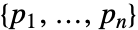 ,得到的置换矩阵
  由
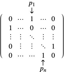
由 ![P〚i,j〛=TemplateBox[{{i, ,, {p, _, j}}}, KroneckerDeltaSeq]](Files/PermutationMatrix.zh/1.png "P〚i,j〛=TemplateBox[{{i, ,, {p, _, j}}}, KroneckerDeltaSeq]") 给出. 这对应于在第
给出. 这对应于在第  行的
行的  列为 1,而在其他地方为零的矩阵.
 - 置换矩阵
 可用于通过
可用于通过  从左侧相乘来置换行,或者通过从右侧乘以它的转置
 ![A.TemplateBox[{P}, Transpose]](Files/PermutationMatrix.zh/3.png "A.TemplateBox[{P}, Transpose]") 来置换列.
来置换列. - 置换矩阵
 是一个正交矩阵,其逆矩阵等价于转置
 ![P^(-1)=TemplateBox[{P}, Transpose]](Files/PermutationMatrix.zh/4.png "P^(-1)=TemplateBox[{P}, Transpose]") .
. - 置换矩阵在矩阵乘法下是闭合的,所以
 也是一个置换矩阵.
 - 置换矩阵的行列式是
 或 1,并且等于 Signature[permv].
 - 为 PermutationMatrix 加速的运算包括:
-
Det 时间 
Dot 时间 
Inverse 时间 
LinearSolve 时间 
- 对于 PermutationMatrix sa,以下属性 "prop" 可以作为 sa["prop"] 访问:
-
"PermutationCycles" 置换矩阵的不相交循环表示 "PermutationList" 置换矩阵的置换列表表示 "WorkingPrecision" 内部使用的精度 "Properties" 支持的属性列表 "Structure" 结构化数组的类型 "StructuredData" 由结构化数组存储的内部数据 "StructuredAlgorithms" 具有结构化数组特殊方法的函数列表 "Summary" 摘要信息,表示为 Dataset - Normal[PermutationMatrix[…]] 将置换矩阵作为普通矩阵给出.
- 可给出以下选项:
-
TargetStructure Automatic 返回的矩阵的结构 WorkingPrecision Infinity 创建元素时使用的精度 - TargetStructure 的可能的设置包括:
-
Automatic 自动选择返回结果的表示形式 "Dense" 用稠密矩阵表示矩阵 "Orthogonal" 用正交矩阵表示矩阵 "Sparse" 用稀疏数组表示矩阵 "Structured" 用结构化数组表示矩阵 "Unitary" 用酉矩阵表示矩阵 - PermutationMatrix[…,TargetStructureAutomatic] 等价于 PermutationMatrix[…,TargetStructure"Structured"].
范例
打开所有单元 关闭所有单元基本范例 (2)
pm = PermutationMatrix[{4, 1, 3, 2}]MatrixForm[pm]Normal[pm]pm = PermutationMatrix[{{0, 1, 0}, {0, 0, 1}, {1, 0, 0}}]MatrixForm[pm]Det[pm]范围 (7)
pm = PermutationMatrix[Cycles[{{1, 4, 3}, {2, 5}}]]MatrixForm[pm]Normal[pm]pm = PermutationMatrix[Cycles[{{1, 4, 3}, {2, 5}}], 7]MatrixForm[pm]从 TwoWayRule 构造一个置换矩阵(互换置换):
pm = PermutationMatrix[2 <-> 6]MatrixForm[pm]Normal[pm]pm = PermutationMatrix[2 <-> 6, 7]MatrixForm[pm]pm = PermutationMatrix[(| | | | | | | | |
| - | - | - | - | - | - | - | - |
| 1 | 0 | 0 | 0 | 0 | 0 | 0 | 0 |
| 0 | 0 | 1 | 0 | 0 | 0 | 0 | 0 |
| 0 | 0 | 0 | 0 | 1 | 0 | 0 | 0 |
| 0 | 0 | 0 | 0 | 0 | 0 | 1 | 0 |
| 0 | 1 | 0 | 0 | 0 | 0 | 0 | 0 |
| 0 | 0 | 0 | 1 | 0 | 0 | 0 | 0 |
| 0 | 0 | 0 | 0 | 0 | 1 | 0 | 0 |
| 0 | 0 | 0 | 0 | 0 | 0 | 0 | 1 |)]MatrixForm[pm]Normal[pm]PermutationMatrix 对象包括提供有关数组信息的属性:
pm = PermutationMatrix[RandomSample[1 ;; 47]]pm["Properties"]"PermutationCycles" 给出底层置换的不相交循环表示:
pm["PermutationCycles"]pm["PermutationList"]pm["WorkingPrecision"]pm["Summary"]属性 "StructuredAlgorithms" 列出具有结构化算法的函数:
pm["StructuredAlgorithms"]pm = PermutationMatrix[Cycles[{{1, 131}, {3, 765}}]]pn = Normal[pm];AbsoluteTiming[Det[pn]]AbsoluteTiming[Det[pm]]AbsoluteTiming[Inverse[pn];]AbsoluteTiming[Inverse[pm];]AbsoluteTiming[Eigenvalues[pn];]AbsoluteTiming[Eigenvalues[pm];]在适当时,结构化算法返回另一个 PermutationMatrix 对象:
perm = {1, 5, 3, 2, 4};
pm = PermutationMatrix[perm]Inverse[pm]pinv = PermutationList[%]perm[[pinv]] == Range[Length[perm]]这等价于 InversePermutation 的结果:
pinv === InversePermutation[perm]perm = PermutationList[RandomPermutation[1*^4]];PermutationMatrix[perm]//ByteCount//AbsoluteTimingInverse[PermutationMatrix[perm]]//ByteCount//AbsoluteTiming普通表示要大得多(80 KB 对 800 MB),并且速度慢得多:
(pnormal = Normal@PermutationMatrix[perm])//ByteCount//AbsoluteTimingInverse[pnormal]//ByteCount//AbsoluteTiming选项 (2)
TargetStructure (1)
PermutationMatrix[Cycles[{{4, 1, 3}}], TargetStructure -> "Dense"]PermutationMatrix[Cycles[{{4, 1, 3}}], TargetStructure -> "Structured"]PermutationMatrix[Cycles[{{4, 1, 3}}], TargetStructure -> "Sparse"]PermutationMatrix[Cycles[{{4, 1, 3}}], TargetStructure -> "Orthogonal"]PermutationMatrix[Cycles[{{4, 1, 3}}], TargetStructure -> "Unitary"]应用 (4)
LUDecomposition 默认使用 PermutationMatrix 作为其返回的置换矩阵:
a = {{4, 9, 2}, {2, 3, 2}, {7, 2, 4}};
{l, u, p, c} = LUDecomposition[a]l.u == p.aMatrixForm /@ {l, u, p}n = 5;
group = DihedralGroup[n];
elems = PermutationMatrix[#, n]& /@ GroupElements[group]Outer[Position[elems, Dot[#1, #2]][[1, 1]]&, elems, elems, 1]这等价于 GroupMultiplicationTable 的结果:
% === GroupMultiplicationTable[group]vec[m_ ? MatrixQ] := Flatten[m, {{2, 1}}]vecPermutationMatrix[p_, q_] := PermutationMatrix[Flatten[Partition[Range[p q], p], {{2, 1}}]]向量置换矩阵将 vec 运算符应用于矩阵及其转置的结果相关联:
p = 4;q = 3;
m1 = Array[, {p, q}];
vec[Transpose[m1]] == vecPermutationMatrix[p, q].vec[m1]向量置换矩阵可以用来表示两个给定矩阵的克罗内克积和逆序的相同矩阵的克罗内克积之间的关系:
r = 4;s = 3;
m2 = Array[, {r, s}];
KroneckerProduct[m1, m2].vecPermutationMatrix[q, s] == vecPermutationMatrix[p, r].KroneckerProduct[m2, m1]快速傅立叶变换 (FFT) 的效率依赖于能够从两个较小的傅立叶矩阵形成一个较大的傅立叶矩阵. 生成大小为 p 和 q 的两个小傅立叶矩阵:
p = 2;
MatrixForm[fmatp = FourierMatrix[p]]q = 3;
MatrixForm[fmatq = FourierMatrix[q]]大小为 p q 的傅立叶矩阵可以表示为四个较简单矩阵的乘积:
fpkp = KroneckerProduct[fmatp, IdentityMatrix[q]];
diag = DiagonalMatrix[Flatten[Table[Exp[(2 π I j k/p q)], {k, 0, p - 1}, {j, 0, q - 1}]]];
fqkp = BlockDiagonalMatrix[ConstantArray[fmatq, p]];
shuffle = PermutationMatrix[Flatten[Partition[Range[p q], p], {{2, 1}}]];
MatrixForm[fmatpq = fpkp.diag.fqkp.shuffle]
证明得到的矩阵等价于 FourierMatrix 的结果:
fmatpq == FourierMatrix[p q]向量的离散傅立叶变换可以通过将傅立叶矩阵的因子连续乘以向量来计算:
data = RandomComplex[1 + I, p q];
res = fpkp.(diag.(fqkp.(shuffle.data)))
结果等价于将 Fourier 应用于向量:
Chop[Max[Abs[res - Fourier[data]]]] == 0属性和关系 (6)
PermutationMatrix[IdentityMatrix[5]]PermutationCycles[%]PermutationMatrix[p<->q] 等价于 PermutationMatrix[Cycles[{{p,q}}]]:
p1 = PermutationMatrix[2 <-> 7]p2 = PermutationMatrix[Cycles[{{2, 7}}]]p1 === p2使用 SparseArray[PermutationMatrix[…]] 得到作为 SparseArray 的表示:
SparseArray[PermutationMatrix[Cycles[{{1, 18, 7}, {2, 5, 4, 10}}]]]perm = RandomSample[1 ;; 5]对置换矩阵预乘等价于对置换列表使用 Part:
v = RandomReal[1, 5];
v[[perm]]pm = PermutationMatrix[perm]pm.v对置换矩阵后乘等价于对置换列表使用 Permute:
Permute[v, perm]v.pmperm = RandomSample[1 ;; 7]pm = PermutationMatrix[perm]Det[pm] == Signature[perm]n = 5;
perm = PermutationMatrix[RandomSample[1 ;; n]];
mat = Array[C, {n, n}];Permanent[perm.mat] == Permanent[mat.perm] == Permanent[mat]//Simplify巧妙范例 (1)
MatrixForm[bi = Normal[SparseArray[{Band[{1, 1}] -> Array[, 5], Band[{1, 2}] -> Array[, 4]}]]]生成具有双对角块的对称块矩阵(Jordan–Wielandt 矩阵):
MatrixForm[biblk = ArrayFlatten[{{0, Transpose[bi]}, {bi, 0}}]]perfectShuffle[n_Integer ? EvenQ] := PermutationMatrix[Flatten[Partition[Range[n], Quotient[n, 2]], {{2, 1}}]]使用“完美洗牌”将 Jordan–Wielandt 矩阵转换为三对角矩阵(Golub–Kahan 三对角矩阵):
pm = perfectShuffle[Length[biblk]];
pm.biblk.Transpose[pm]//MatrixFormSingularValueList[bi2 = Normal[SparseArray[{Band[{1, 1}] -> {1., 3., 5., 7., 9., 11., 13.}, Band[{1, 2}] -> {2., 4., 6., 8., 10., 12.}}]]]pm = perfectShuffle[2Length[bi2]];Select[Eigenvalues[pm.ArrayFlatten[{{0, Transpose[bi2]}, {bi2, 0}}].Transpose[pm]], Positive]文本
Wolfram Research (2022),PermutationMatrix,Wolfram 语言函数,https://reference.wolfram.com/language/ref/PermutationMatrix.html (更新于 2024 年).
CMS
Wolfram 语言. 2022. "PermutationMatrix." Wolfram 语言与系统参考资料中心. Wolfram Research. 最新版本 2024. https://reference.wolfram.com/language/ref/PermutationMatrix.html.
APA
Wolfram 语言. (2022). PermutationMatrix. Wolfram 语言与系统参考资料中心. 追溯自 https://reference.wolfram.com/language/ref/PermutationMatrix.html 年