

RootMeanSquare
RootMeanSquare[list]
给出 list 中值的均方根.
RootMeanSquare[dist]
给出分布 dist 的均方根.
更多信息
- RootMeanSquare 测量数据规模或分布.
- RootMeanSquare[list] 给出第二样本矩的平方根.
- 对于 {x1,x2,…,xn},均方根由
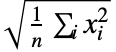 给出.
- RootMeanSquare 处理数值和符号数据.
- RootMeanSquare[{{x1,y1,…},{x2,y2,…},…}] 给出 {RootMeanSquare[{x1,x2,…}],RootMeanSquare[{y1,y2,…}]}.
- RootMeanSquare[dist] 等价于 Sqrt[Expectation[x2,xdist]].
范例
打开所有单元 关闭所有单元基本范例 (3)
一个列表的 RootMeanSquare :
RootMeanSquare[ {a, b, c, d}]矩阵列的 RootMeanSquare:
RootMeanSquare[{{1, 2}, {5, 10}, {5, 2}, {4, 8}}]参数分布的 RootMeanSquare:
RootMeanSquare[LogNormalDistribution[0, 1]]范围 (14)
数据 (10)
RootMeanSquare[{1, 2, 3, 4}]RootMeanSquare[{π, E, 2}]RootMeanSquare[{1., 2., 3., 4.}]RootMeanSquare[N[{1, 2, 3, 4}, 30]]矩阵的 RootMeanSquare 逐列给出均值:
RootMeanSquare[(| | |
| --- | --- |
| a11 | a12 |
| a21 | a22 |)]RootMeanSquare[RandomReal[1, 10 ^ 7]]RootMeanSquare[RandomReal[1, {10 ^ 6, 3}]]可以像使用稠密数组一样使用 SparseArray 数据:
RootMeanSquare[SparseArray[{{1} -> 1, {2} -> 7}]]RootMeanSquare[SparseArray[{{1, 1} -> 1, {2, 1} -> 2, {2, 2} -> 3}]]对于 SparseArray 的计算结果:
sp = SparseArray[{{i_, i_} :> i, {i_, j_} /; j == i + 1 :> i - 1}, {100, 10}]RootMeanSquare[sp]WeightedData 的 RootMeanSquare:
RootMeanSquare[WeightedData[{1, 2, 3}, {Subscript[w, 1], Subscript[w, 2], Subscript[w, 3]}]]data = {8, 3, 5, 4, 9, 1, 4, 2, 2, 3};
weights = {0.15, 0.09, 0.12, 0.10, 0.16, 0.3, 0.11, 0.08, 0.08, 0.09};RootMeanSquare[WeightedData[data, weights]]e = {1.0, 2.1, 3.2, 4.5, 5.7};
ci = {0, 0, 0, 1, 0};RootMeanSquare[EventData[e, ci]]RootMeanSquare[TemporalData[TimeSeries, {{{2.3, 1.2, 6.7, 5.8, 7.1, 4.6}}, {{0, 5, 1}}, 1, {"Discrete", 1},
{"Discrete", 1}, 1, {}}, False, 10.]]RootMeanSquare[TemporalData[TimeSeries, {{{2.3, 1.2, 6.7, 5.8, 7.1, 4.6}}, {{0, 5, 1}}, 1, {"Discrete", 1},
{"Discrete", 1}, 1, {}}, False, 10.]["Values"]]涉及量的数据的 RootMeanSquare:
data = Quantity[RandomReal[1, 6], "Meters"]RootMeanSquare[data]分布和过程 (4)
求单变量分布的 RootMeanSquare:
RootMeanSquare[BinomialDistribution[n, p]]RootMeanSquare[NormalDistribution[μ, σ]]RootMeanSquare[MultinomialDistribution[n, {Subscript[m, 1], Subscript[m, 2]}]]RootMeanSquare[BinormalDistribution[{Subscript[μ, 1], Subscript[μ, 2]}, {σ1, σ2}, ρ]]导出分布的 RootMeanSquare:
RootMeanSquare[TransformedDistribution[x^2, xNormalDistribution[μ, σ]]]RootMeanSquare[ProbabilityDistribution[(Sqrt[2] / π)(1 / (1 + (x - 2)^4)), {x, -∞, ∞}]]data = RandomVariate[NormalDistribution[], 10 ^ 3];RootMeanSquare[HistogramDistribution[data]]含有量的分布的 RootMeanSquare:
RootMeanSquare[QuantityDistribution[MaxwellDistribution[σ], "Meters" / "Seconds"]]RootMeanSquare[EmpiricalDistribution[QuantityArray[RandomChoice[{0, 5}, 1000], "Volts"]]]随机过程的 RootMeanSquare:
RootMeanSquare[BrownianBridgeProcess[a, b][t]]Plot[Evaluate[% /. {a -> 3, b -> 5}], {t, 3, 5}, PlotRange -> All]应用 (3)
data = {{1, 2.9}, {2, 5.0}, {3, 7.1}, {4, 8.9}, {5, 10.9}, {6, 13.1}, {7, 14.9}, {8, 16.8}, {9, 18.5}, {10, 22.2}};f[x_] = Fit[data, {1, x}, x]RootMeanSquare[data[[All, 2]] - Map[f, data[[All, 1]]]]f[t_] := Sin[5 t] + Cos[7t] / 12ts = TimeSeries[Table[f[t], {t, 0, 2Pi, 0.01}]]ListPlot[ts]RootMeanSquare[ts]Sqrt[Integrate[f[t] ^ 2, {t, 0, 2Pi}] / (2Pi)]N[%]heights = Quantity[{134, 143, 131, 140, 145, 136, 131, 136, 143, 136, 133, 145, 147,
150, 150, 146, 137, 143, 132, 142, 145, 136, 144, 135, 141}, "Centimeters"];ListPlot[heights, Filling -> Axis, AxesLabel -> Automatic](rms = RootMeanSquare[heights])//NListPlot[{heights, {{0, rms}, {Length[heights], rms}}}, Joined -> {False, True}, Filling -> Axis, AxesLabel -> Automatic]属性和关系 (7)
RootMeanSquare 是数据平方的 Mean 的平方根:
data = RandomReal[10, 10];Sqrt[Mean[data ^ 2]]RootMeanSquare[data]RootMeanSquare 等价于经过缩放的 Norm:
data = RandomReal[10, 10];Norm[data] / Sqrt[Length[data]]RootMeanSquare[data]偏差的 RootMeanSquare 等价于经过缩放的 StandardDeviation:
data = RandomReal[10, 10];StandardDeviation[data]Sqrt[(Length[data] - 1) / Length[data]]RootMeanSquare[data - Mean[data]]偏差的 RootMeanSquare 是 CentralMoment 的平方根:
data = RandomReal[10, 10];CentralMoment[data, 2]//SqrtRootMeanSquare[data - Mean[data]]RootMeanSquare 是距 Mean 的经过缩放的 EuclideanDistance:
data = RandomReal[10, 10];mean = Mean[data]RootMeanSquare[data - mean]EuclideanDistance[data, mean] / Sqrt[Length[data]]随机变量的 RootMeanSquare 是 Expectation 的平方根:
dist = GammaDistribution[α, β];Sqrt[Expectation[x ^ 2, xdist]]RootMeanSquare[dist]RootMeanSquare 是规模的度量:
𝒟 = NormalDistribution[a, σ];RootMeanSquare[𝒟]Table[Plot[PDF[𝒟 /. {a -> 1}, x], {x, -4, 6}, PlotRange -> {0, 0.4}, Filling -> Axis, Ticks -> {Automatic, None}, PlotLabel -> Row[{"SuperscriptBox[σ, 2] = ", σ^2}]], {σ, {1, 1.5, 2}}]文本
Wolfram Research (2007),RootMeanSquare,Wolfram 语言函数,https://reference.wolfram.com/language/ref/RootMeanSquare.html (更新于 2017 年).
CMS
Wolfram 语言. 2007. "RootMeanSquare." Wolfram 语言与系统参考资料中心. Wolfram Research. 最新版本 2017. https://reference.wolfram.com/language/ref/RootMeanSquare.html.
APA
Wolfram 语言. (2007). RootMeanSquare. Wolfram 语言与系统参考资料中心. 追溯自 https://reference.wolfram.com/language/ref/RootMeanSquare.html 年