

SingularValueDecomposition
给出一个数值矩阵 m 的奇异值分解,形式为矩阵列表 {u,σ,v},其中 σ 是一个对角矩阵,m 可以写为 u.σ.ConjugateTranspose[v].
SingularValueDecomposition[{m,a}]
给出 m 相对于 a 的广义奇异值分解.
SingularValueDecomposition[m,spec]
给出与 spec 指定的最大奇异值相关的奇异值分解.
更多信息和选项
- 矩阵 m 可以是矩形.
- σ 的对角线元素是 m 的奇异值.
- SingularValueDecomposition 将去掉 SingularValueList 设为零的奇异值.
- 选项 Tolerance 可以在 SingularValueList 中使用来决定哪些奇异值被考虑为零. »
- u 和 v 为列正交矩阵,其转置可被视为正交向量的列表.
- SingularValueDecomposition[{m,a}] 给出 {{u,ua},{w,wa},v} 矩阵列表,这样 m 可以写为 u.w.ConjugateTranspose[v],a 可以写为 ua.wa.ConjugateTranspose[v]. »
- 第二个参数 spec 可以采用以下设置:
-
k 返回与前 k 个最大奇异值对应的分解 UpTo[k] 返回前 k 个最大奇异值中可获得的分解 "Thin" 返回使用 Min[Dimensions[m]] 个最大奇异值的"薄"奇异值分解 - 采用设置 TargetStructure->"Structured" 时,SingularValueDecomposition[m] 以结构化矩阵的形式返回矩阵 {u,σ,v}.
范例
打开所有单元 关闭所有单元基本范例 (3)
{u, σ, v} = SingularValueDecomposition[(| | |
| - | - |
| 1 | 2 |
| 1 | 2 |)]u.σ.Transpose[v]//MatrixForm{u, σ, v} = SingularValueDecomposition[(| | |
| --- | --- |
| 0.5 | 1 |
| 2 | 2.5 |)]σ//MatrixFormu.σ.Transpose[v]{u, σ, v} = SingularValueDecomposition[(| | |
| --- | --- |
| 1.2 | 3.4 |
| 5.6 | 7.8 |
| 9.0 | 1.2 |)]MatrixForm /@ {u, σ, v}u.σ.Transpose[v]//MatrixForm范围 (18)
基础用法 (7)
SingularValueDecomposition[(| | | |
| --- | --- | --- |
| 1.1 | 1.3 | 2.1 |
| 2.2 | 2.2 | 3.3 |
| 3.3 | -3 | 4.7 |)]MatrixForm /@ %MatrixForm /@ SingularValueDecomposition[(| | |
| ----------- | ----------- |
| 0.5 + 0.5 I | 1.1 |
| -I | 3.2 - 4.5 I |)]SingularValueDecomposition[{{2, 3}, {0, 2}}]MatrixForm /@ SingularValueDecomposition[MatrixExp[RandomReal[1, {2, 2}, WorkingPrecision -> 12]]]Simplify[SingularValueDecomposition[(| | |
| --------- | - |
| Sqrt[2] x | 1 |
| 0 | 1 |)], x∈ℝ]mat = RandomReal[{0, 9}, {1000, 1000}];AbsoluteTiming[SingularValueDecomposition[mat];]MatrixForm /@ SingularValueDecomposition[(| | | |
| --- | --- | --- |
| 1.1 | 2 | 5 |
| 3 | -11 | 4.2 |)]奇异值的子集 (5)
m = (| | | | | |
| --- | --- | ---- | ----- | ------ |
| 0.5 | 0.5 | 0.5 | 0 | 0 |
| 1. | 2. | 4. | 8. | 0 |
| 1.5 | 4.5 | 13.5 | 40.5 | 121.5 |
| 0 | 8. | 32. | 128. | 512. |
| 0 | 0 | 62.5 | 312.5 | 1562.5 |);{u, σ, v} = SingularValueDecomposition[m, 3];
Map[MatrixForm, {u, σ, v}]//Chopm - u.σ.ConjugateTranspose[v]//MatrixFormMatrixForm /@ SingularValueDecomposition[m, -3]m = {{0.5, 1., 1.5}, {2., 2.5, 3.}, {3.5, 4., 4.5}};{ut, σt, vt} = SingularValueDecomposition[m, MatrixRank[m]]m == ut.σt.Transpose[vt]MatrixForm /@ SingularValueDecomposition[m]m = {{1.2, 3.4}, {5.6, 7.8}, {9.0, 1.2}};MatrixForm /@ ({ut, σt, vt} = SingularValueDecomposition[m, "Thin"])
SquareMatrixQ[σt]Length[σt] == Min[Dimensions[m]]m == ut.σt.Transpose[vt]
MatrixForm /@ SingularValueDecomposition[m]求与三个最大奇异值相关的分解,或如果数量少的话则计算与奇异值数量一样的分解:
MatrixForm /@ SingularValueDecomposition[(| | | | | |
| --- | --- | --- | --- | --- |
| 0.5 | 1. | 1.5 | 2. | 2.5 |
| 2. | 2.5 | 3. | 3.5 | 4. |
| 3.5 | 4. | 4.5 | 5. | 5.5 |
| 4. | 4.5 | 5. | 5.5 | 6. |), UpTo[3]]mat = {{(7/2), 0, (1/2), 0}, {0, 3, 0, 1}, {(1/2), 0, (7/2), 0}, {0, 1, 0, 3}};SingularValueList[mat]MatrixForm /@ SingularValueDecomposition[mat, 3]MatrixForm /@ SingularValueDecomposition[mat, -3]广义奇异值分解 (2)
m = {{1.5, 1.3}, {3.1, 2.2}};a = {{1.1, 5.1}, {4.2, 3.4}};{{u, ua}, {σ, σa}, v} = SingularValueDecomposition[{m, a}];
MatrixForm /@ {u, ua, σ, σa, v}{m == u.σ.ConjugateTranspose[v], a == ua.σa.ConjugateTranspose[v]}m = (| | |
| ---------------------------------------- | ---------------------------------------- |
| 4.641175490606916 + 7.207263282382337 I | 2.522671922520866 + 8.989217121399136 I |
| 4.114478069008367 + 7.010706036954508 I | 8.95961276370625 + 3.569738897382109 I |
| 4.405169936758572 + 4.4509297530197465 I | 9.145107926643146 + 6.3767022076415465 I |);a = (| | |
| --------------------------------------- | ---------------------------------------- |
| 7.341517476299638 + 9.810565178638917 I | 8.24181899398409 + 3.4570598473462972 I |
| 7.775955216608212 + 1.68269060515731 I | 3.944961113408187 + 1.4889990223210265 I |
| 6.431377195364613 + 6.245150387114993 I | 7.026661544586792 + 1.0790173484547747 I |);{{u, ua}, {σ, σa}, v} = SingularValueDecomposition[{m, a}];
MatrixForm /@ {u, ua, σ, σa, v}//Chop{m == u.σ.ConjugateTranspose[v], a == ua.σa.ConjugateTranspose[v]}特殊矩阵 (4)
SparseArray[{{1, 3} -> 2, {2, 2} -> 3, {3, 1} -> 1, {4, 2} -> 5}, {4, 4}]MatrixForm /@ SingularValueDecomposition[%]Block[{n = 200}, SparseArray[{{i_, i_} -> -2.,
{i_, j_} /; Abs[i - j] == 1 -> 1.}, n]]{u, σ, v} = SingularValueDecomposition[%, 3, Method -> {"Arnoldi", MaxIterations -> 3000}];ListPlot[Transpose[v]]SymmetrizedArray[{{1, 1} -> 2, {1, 2} -> 1}, {2, 2}, Symmetric[All]]SingularValueDecomposition[%]QuantityArray[{{1, 2}, {3, 4}}, {"Meters", "Meters"}]MatrixForm /@ SingularValueDecomposition[%]//N{u, σ, v} = SingularValueDecomposition[IdentityMatrix[3]];
Map[MatrixForm, {u, σ, v}]u.σ.Transpose[v] == IdentityMatrix[3]

ui = vi = IdentityMatrix[3];
ui.σ.Transpose[vi] == IdentityMatrix[3]
HilbertMatrix 的奇异值分解:
svd = SingularValueDecomposition[HilbertMatrix[3]];
MatrixForm /@ N[svd]
选项 (3)
TargetStructure (2)
ma = RandomReal[1, {6, 4}]设 TargetStructure->"Dense" 时,SingularValueDecomposition 的结果是三个稠密矩阵组成的列表:
SingularValueDecomposition[ma, TargetStructure -> "Dense"]设 TargetStructure->"Structured" 时,SingularValueDecomposition 的结果是一个列表,其中含有两个 OrthogonalMatrix 对象和一个 DiagonalMatrix:
SingularValueDecomposition[ma, TargetStructure -> "Structured"]ma = RandomComplex[1 + I, {6, 4}]设 TargetStructure->"Dense" 时,SingularValueDecomposition 的结果是三个稠密矩阵组成的列表:
SingularValueDecomposition[ma, TargetStructure -> "Dense"]设 TargetStructure->"Structured" 时,SingularValueDecomposition 的结果是一个列表,其中含有两个 UnitaryMatrix 对象和一个 DiagonalMatrix:
SingularValueDecomposition[ma, TargetStructure -> "Structured"]Tolerance (1)
m = {{1, 0}, {1, 10^-14}};SingularValueDecomposition[N[m]]SingularValueDecomposition[N[m], Tolerance -> 10^-15]SingularValueDecomposition[N[m, 20]]应用 (11)
奇异值分解的几何学 (5)


m = (| | |
| ---- | ----- |
| 0.76 | -0.32 |
| 0.26 | -0.75 |);
MatrixForm /@ ({u, σ, v} = SingularValueDecomposition[m]) 的动作是一个旋转,并像在这种情况下可能是发生在
 轴上的一个反射:
ParametricPlot[{Transpose[v].{Cos[θ], Sin[θ]}, {Cos[θ], Sin[θ]}}, {θ, 0, 2π}, IconizedObject[«Plot Options»]]
ParametricPlot[{σ.Transpose[v].{Cos[θ], Sin[θ]}, Transpose[v].{Cos[θ], Sin[θ]}}, {θ, 0, 2π}, IconizedObject[«Plot Options»]] 的动作是一个旋转,并且可能是——尽管在这种情况下并不是——目标空间中的反射:
ParametricPlot[{u.σ.Transpose[v].{Cos[θ], Sin[θ]}, σ.Transpose[v].{Cos[θ], Sin[θ]}}, {θ, 0, 2π}, IconizedObject[«Plot Options»]]
m = (| | |
| ---- | ---- |
| 0.96 | 0.49 |
| 0.3 | 0.83 |
| 0.72 | 0.39 |);
MatrixForm /@ ({u, σ, v} = SingularValueDecomposition[m])

addArrows[inMat_, outMat_] := Graphics3D[...]
Show[ParametricPlot3D[{σ.Transpose[v].{Cos[θ], Sin[θ]}, Append[Transpose[v].{Cos[θ], Sin[θ]}, 0]}, {θ, 0, 2π}, IconizedObject[«Plot Options»]], addArrows[σ.Transpose[v], Append[Transpose[v], {0, 0}]]]
Show[ParametricPlot3D[{u.σ.Transpose[v].{Cos[θ], Sin[θ]}, σ.Transpose[v].{Cos[θ], Sin[θ]}}, {θ, 0, 2π}, IconizedObject[«Plot Options»]], addArrows[u.σ.Transpose[v], σ.Transpose[v]]]
m = {{1.1, -1.3}, {1.2, 2.5}};
MatrixForm /@ ({u, σ, v} = SingularValueDecomposition[m])


{{u1, u2}, {v1, v2}} = {Transpose[u], Transpose[v]};


Maximize[Norm[m.x], x∈Circle[]]


Minimize[Norm[m.x], x∈Circle[]]


ParametricPlot[m.{Cos[t], Sin[t]}, {t, 0, 2Pi}, Epilog -> {Thick, {RGBColor[0.880722, 0.611041, 0.142051], Line[{{0, 0}, m.v1}], Dashed, Line[{{0, 0}, v1}]}, {RGBColor[0.560181, 0.691569, 0.194885], Line[{{0, 0}, m.v2}], Dashed, Line[{{0, 0}, v2}]}, {RGBColor[0.368417, 0.506779, 0.709798], Dashed, Circle[]}}, Ticks -> {{-1.5, 1.5}, Automatic}]


Maximize[Norm[x.m], x∈Circle[]]


Minimize[Norm[x.m], x∈Circle[]]


ParametricPlot[{Cos[t], Sin[t]}.m, {t, 0, 2Pi}, Epilog -> {Thick, {RGBColor[0.880722, 0.611041, 0.142051], Line[{{0, 0}, u1.m}], Dashed, Line[{{0, 0}, u1}]}, {RGBColor[0.560181, 0.691569, 0.194885], Line[{{0, 0}, u2.m}], Dashed, Line[{{0, 0}, u2}]}, {RGBColor[0.368417, 0.506779, 0.709798], Dashed, Circle[]}}, Ticks -> {{-1.5, 1.5}, Automatic}]
m = (| | |
| --------- | --------- |
| 3 | 3 |
| 4 | -4 |
| 3 Sqrt[3] | 3 Sqrt[3] |);
MatrixForm /@ ({u, σ, v} = SingularValueDecomposition[m])


{{u1, u2, u3}, {v1, v2}} = {Transpose[u], Transpose[v]};


Maximize[Norm[m.x], x∈Circle[]]


Minimize[Norm[m.x], x∈Circle[]]


Show[ParametricPlot3D[m.{Cos[t], Sin[t]}, {t, 0, 2Pi}], Graphics3D[{RGBColor[0.880722, 0.611041, 0.142051], Tube[{{0, 0, 0}, m.v1}], RGBColor[0.560181, 0.691569, 0.194885], Tube[{{0, 0, 0}, m.v2}]}]]


Maximize[Norm[x.m], x∈Sphere[]]

Minimize[Norm[x.m], x∈Sphere[]]


Maximize[{Norm[x.m], u1.x == 0}, x∈Sphere[]]


ParametricPlot[{Cos[p]Sin[t], Sin[p]Sin[t], Cos[t]}.m, {p, 0, 2Pi}, {t, 0, π}, Epilog -> {Thick, {RGBColor[0.880722, 0.611041, 0.142051], Arrow[{{0, 0}, u1.m}]}, {RGBColor[0.560181, 0.691569, 0.194885], Arrow[{{0, 0}, u2.m}]}, {RGBColor[0.922526, 0.385626, 0.209179], AbsolutePointSize[5], Point[u3.m]}}]
m = (| | | |
| ------ | ------ | ---- |
| -0.069 | 0.35 | 0.98 |
| 0.50 | -0.072 | 0.64 |
| 0.92 | 0.93 | 0.15 |);
MatrixForm /@ ({u, σ, v} = SingularValueDecomposition[m])


{{u1, u2, u3}, {v1, v2, v3}} = {Transpose[u], Transpose[v]};


Maximize[Norm[m.x], x∈Sphere[]]


Maximize[{Norm[m.x], x.v1 == 0}, x∈Sphere[]]


Minimize[Norm[m.x], x∈Sphere[]]


{Show[ParametricPlot3D[{Cos[p] Sin[t], Sin[p] Sin[t], Cos[t]}, {p, 0, 2 Pi}, {t, 0, π}, IconizedObject[«Plot Options»]], Graphics3D[Riffle[{RGBColor[0.5, 0, 0.5], RGBColor[0.560181, 0.691569, 0.194885], RGBColor[0.922526, 0.385626, 0.209179]}, Arrow[Tube[{{0, 0, 0}, #}]]& /@ Transpose[v]]], ImageSize -> 250], Show[ParametricPlot3D[m.{Cos[p] Sin[t], Sin[p] Sin[t], Cos[t]}, {p, 0, 2 Pi}, {t, 0, π}, IconizedObject[«Plot Options»]], Graphics3D[Riffle[{RGBColor[0.5, 0, 0.5], RGBColor[0.560181, 0.691569, 0.194885], RGBColor[0.922526, 0.385626, 0.209179]}, Arrow[Tube[{{0, 0, 0}, m.#}]]& /@ Transpose[v]]], ImageSize -> 250]}


Maximize[Norm[x.m], x∈Sphere[]]


Maximize[{Norm[x.m], x.u1 == 0}, x∈Sphere[]]


Minimize[Norm[x.m], x∈Sphere[]]


{Show[ParametricPlot3D[{Cos[p] Sin[t], Sin[p] Sin[t], Cos[t]}, {p, 0, 2 Pi}, {t, 0, π}, IconizedObject[«Plot Options»]], Graphics3D[Riffle[{RGBColor[0.5, 0, 0.5], RGBColor[0.560181, 0.691569, 0.194885], RGBColor[0.922526, 0.385626, 0.209179]}, Arrow[Tube[{{0, 0, 0}, #}]]& /@ Transpose[u]]], ImageSize -> 250], Show[ParametricPlot3D[{Cos[p] Sin[t], Sin[p] Sin[t], Cos[t]}.m, {p, 0, 2 Pi}, {t, 0, π}, IconizedObject[«Plot Options»]], Graphics3D[Riffle[{RGBColor[0.5, 0, 0.5], RGBColor[0.560181, 0.691569, 0.194885], RGBColor[0.922526, 0.385626, 0.209179]}, Arrow[Tube[{{0, 0, 0}, #.m}]]& /@ Transpose[u]]], ImageSize -> 250]}最小二乘和曲线拟合 (6)
如果线性方程组  没有解,最好的近似解是最小二乘解. 这就是
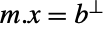 的解,其中
 是
 在
 的列空间上的正交投影,可以使用奇异值分解来计算. 思考以下
 和
 :
m = (| | |
| - | -- |
| 1 | 2 |
| 3 | -4 |
| 1 | -1 |);
b = {0, -2, 1};LinearSolve[m, b]


u = First[SingularValueDecomposition[m, MatrixRank[m]]];
u//N//MatrixForm


bPerp = u.Transpose[u].b//FullSimplify


{b1, b2} = Transpose[u](Transpose[u].b);
Graphics3D[...]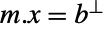
LinearSolve[m, bPerp]使用 LeastSquares 验证结果:
LeastSquares[m, b]

m = (| | | |
| ------------ | ----------- | ------------ |
| 4. + 0.5 I | 3. + 0.5 I | 4.5 + 0.5 I |
| 3.5 + 0.5 I | 4. + 0.5 I | 3.5 + 0.5 I |
| -3. - 0.5 I | -5. - 0.5 I | -2.5 - 0.5 I |);
b = {0, -2, 1 + I};MatrixForm /@ ({u, σ, v} = SingularValueDecomposition[m, MatrixRank[m]])
x = v.Inverse[σ].ConjugateTranspose[u].b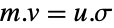



m.x == u.ConjugateTranspose[u].b因此,正如 LeastSquares 所证实的一样, 是最小二乘问题的解:
x == LeastSquares[m, b]求以下  和
 的最小二乘问题的两种不同方法:仅使用奇异值分解的
 矩阵投影到
 的列空间,以及使用完全分解的直接解求解法. 比较并解释结果:
m = (|   |   |   |
| - | - | - |
| 1 | 5 | 4 |
| 2 | 6 | 4 |
| 3 | 7 | 4 |
| 4 | 8 | 4 |);
b = {0, -2, 1, 2};{u, σ, v} = SingularValueDecomposition[m, MatrixRank[m]]//FullSimplify;


bPerp = u.Transpose[u].b//FullSimplify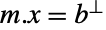
xPerp = LinearSolve[m, bPerp]


x = v.Inverse[σ].Transpose[u].b//FullSimplify虽然 x 和 xPerp 不同,但都可求解最小二乘问题,因为 m.x==m.xPerp:
m.xPerp == m.x这两个解的不同之处在于 NullSpace[m] 的一个元素:
x - xPerpNullSpace[m]请注意,LeastSquares[m,b] 使用直接方法给出结果:
x == LeastSquares[m, b]


m = {{1, 1}, {1, 2}, {1, 3}};
b = {{7, 1}, {7, 2}, {8, 3}};
{u, σ, v} = SingularValueDecomposition[m, MatrixRank[m]];
v.Inverse[σ].Transpose[u].b//FullSimplify
使用 LeastSquares[m,b] 也可以得到这个结果:
LeastSquares[m, b]使用 Minimize 验证答案:
Minimize[Norm[m.{{w, x}, {y, z}} - b, "Frobenius"], {w, x, y, z}]SingularValueDecomposition 可用于找到数据的最佳拟合曲线. 思考下列数据:
data = IconizedObject[«Data»];
ListPlot[data]

{x, y} = Extract[data, {{All, 1}, {All, 2}}];


m = Map[x |-> {1, x}, x];

{u, σ, v} = SingularValueDecomposition[m, 2];
{a, b} = v.Inverse[σ].Transpose[u].y
使用 Fit 验证系数:
Fit[data, {1, s}, s]Show[Plot[a + b x, {x, 0, 1}], ListPlot[data]]data = IconizedObject[«Data»];
ListPlot[data]

{x, y} = Extract[data, {{All, 1}, {All, 2}}];


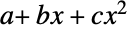
m = DesignMatrix[data, {1, , ^ 2}, ];


{u, σ, v} = SingularValueDecomposition[m, 3];
{a, b, c} = v.Inverse[σ].Transpose[u].y
使用 Fit 验证系数:
Fit[data, {1, s, s ^ 2}, s]Show[Plot[a + b x + c x ^ 2, {x, 0, 3}], ListPlot[data, IconizedObject[«plot options»]]]属性和关系 (13)
m 的奇异值分解 {u,σ,v} 将 m 分解为 u.σ.ConjugateTranspose[v]:
m = RandomComplex[1 + I, {3, 4}];
{u, σ, v} = SingularValueDecomposition[m];
Chop[m - u.σ.ConjugateTranspose[v]]
如果 a 是具有分解 {u,σ,v} 的 n×m 矩阵,则 u 是 n×n 矩阵:
n = 5;m = 3;a = RandomReal[1, {n, m}];
{u, σ, v} = SingularValueDecomposition[a];
Dimensions[u] == {n, n}Dimensions[v] == {m, m}Dimensions[σ] == {n, m}SingularValueDecomposition[m] 是由  和
 的特征值分解构建的:
m = (| | | |
| ---- | --- | ---- |
| -5.2 | 0 | -5 |
| 1.7 | 5.4 | -4.3 |);{u, Σ, v} = SingularValueDecomposition[m];计算 EigenvalueDecomposition[m.ConjugateTranspose[m]]:
{Subscript[t, L], Subscript[d, L]} = EigenvalueDecomposition[m . ConjugateTranspose[m]];

{u//MatrixForm, Subscript[t, L]//MatrixForm}
{Subscript[t, R], Subscript[d, R]} = EigenvalueDecomposition[ConjugateTranspose[m].m];

{v//MatrixForm, Subscript[t, R]//MatrixForm}


MatrixForm /@ {Σ, Sqrt[Subscript[d, L]]}
m = {{0.74, 0.43, 0.28}, {0.63, 0.74, 0.4}, {0.47000000000000003, 0.9400000000000001, 0.55}};v1 = ArgMax[Norm[m.x], x∈Sphere[{0, 0, 0}]]每个后续向量都是一个最大化器,其约束条件是它垂直于所有先前的向量:
v2 = ArgMax[{Norm[m.x], v1.x == 0}, x∈Sphere[{0, 0, 0}]]v3 = ArgMax[{Norm[m.x], v1.x == 0 && v2.x == 0}, x∈Sphere[{0, 0, 0}]]将  与 SingularValueDecomposition 求得的
 进行比较;除符号之外其他是一样的:
{u, σ, v} = SingularValueDecomposition[m];
MatrixForm /@ {Transpose[{v1, v2, v3}], v}
u1 = ArgMax[Norm[x.m], x∈Sphere[{0, 0, 0}]];
u2 = ArgMax[{Norm[x.m], u1.x == 0}, x∈Sphere[{0, 0, 0}]];
u3 = ArgMax[{Norm[x.m], u1.x == 0 && u2.x == 0}, x∈Sphere[{0, 0, 0}]];
MatrixForm /@ {Transpose[{u1, u2, u3}], u}
{Diagonal[σ], Norm /@ {m.v1, m.v2, m.v3}, Norm /@ {u1.m, u2.m, u3.m}}//MatrixForm


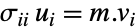
m = RandomInteger[1, {3, 4}];
{u, σ, v} = SingularValueDecomposition[m];
Table[σ[[i, i]]u[[All, i]] == m.v[[All, i]], {i, 3}]//FullSimplify


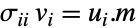
Table[σ[[i, i]]v[[All, i]] == u[[All, i]].m, {i, 3}]//FullSimplify如果 m 是方阵, 的对角元素的乘积等于 Abs[Det[m]]:
m = RandomReal[1, {5, 5}];
Times@@Diagonal[SingularValueDecomposition[m][[2]]] == Abs[Det[m]]


m = (| | | |
| ------------------- | ------------------- | -------------------- |
| 0 | -0.2785693493596917 | -0.12624545596692704 |
| 0.2785693493596917 | 0 | -0.08798023011262301 |
| 0.12624545596692704 | 0.08798023011262301 | 0 |);
NormalMatrixQ[m]除非  是半正定的并且是埃尔米特矩阵,否则向量将以不同的顺序出现:
{u, σ, v} = SingularValueDecomposition[m]//Chop;
{u//MatrixForm, v//MatrixForm} 的对角线项等于 Abs[Eigenvalues[m]]:
Diagonal[σ] == Chop[Abs[Eigenvalues[m]]]对于正定的埃尔米特  ,SingularValueDecomposition 与 EigenvalueDecomposition 是一致的:
m = (| | | |
| -------------------------------------------- | -------------------------------------------- | -------------------------------------------- |
| 3.830367325120047 + 0. I | 0.07350793635153963 - 0.12698026356721126 I | -0.7939695217640885 - 0.002520762074857519 I |
| 0.07350793635153963 + 0.12698026356721126 I | 2.4790235245220367 + 0. I | -0.046544276125373374 - 0.5373197314346221 I |
| -0.7939695217640885 + 0.002520762074857519 I | -0.046544276125373374 + 0.5373197314346221 I | 1.042188083119043 + 0. I |);
{u, σ, v} = SingularValueDecomposition[m];
{t, d} = EigenvalueDecomposition[m];
PositiveDefiniteMatrixQ[m] && HermitianMatrixQ[m]

u - v//Chop

Abs[t / u]


σ == dMatrixRank[m] 等于非零奇异值的数量:
m  = RandomInteger[1, {3, 3}];
{u, σ, v} = SingularValueDecomposition[m];
MatrixRank[m] == Length[Select[Diagonal[σ], x |-> x > 0]]
只保留非零奇异值的紧凑分解可计算 PseudoInverse[m]:
m = {{1, 2, 3}, {4, 5, 6}, {7, 8, 9}};{u, σ, v} = SingularValueDecomposition[m, MatrixRank[m]];


PseudoInverse[m] == v.Inverse[σ].ConjugateTranspose[u]//FullSimplify作为两个向量的外积的矩阵 m 可有 MatrixRank[m]==1:
x1 = {1, 2, 3};x2 = {4, 5};
m = Outer[Times, x1, x2]MatrixRank[m]{u, σ, v} = SingularValueDecomposition[m, 1]σ[[1, 1]] == Norm[x1]Norm[x2]{u[[All, 1]] == (x1/Norm[x1]), v[[All, 1]] == (x2/Norm[x2])}SingularValueDecomposition[{m,a}] 将 m 分解为 u.w.ConjugateTranspose[v]:
m = RandomComplex[1 + I, {3, 4}];
a = RandomComplex[1 + I, {2, 4}];
{{u, ua}, {w, wa}, v} = SingularValueDecomposition[{m, a}];
Chop[m - u.w.ConjugateTranspose[v]]
其将 a 分解为 ua.wa.ConjugateTranspose[v]:
Chop[a - ua.wa.ConjugateTranspose[v]]SingularValueDecomposition[{m,a}] 可与 Eigensystem[{m.m,a.a}] 关联:
m = (| | | |
| ------------------------------------------ | ------------------------------------------- | ------------------------------------------ |
| 0.9753346860069796 + 0.32225791006850857 I | 0.8493715230848708 + 0.39224803196754077 I | 0.5839367017062629 + 0.11364379814173331 I |
| 0.8359555932254314 + 0.7712743289239168 I | 0.48928975439484756 + 0.48056805668910774 I | 0.3042001847125009 + 0.11991764017567741 I |
| 0.4727880193915137 + 0.9358524506075876 I | 0.9540225347992926 + 0.545522455352986 I | 0.1542301183700603 + 0.02063002461235164 I |);
a = (| | | |
| --------------------------------------------- | ------------------------------------------ | ------------------------------------------- |
| 0.0002671678119234855 + 0.17886262704796918 I | 0.23822746561953023 + 0.6255181037100543 I | 0.8983010971084864 + 0.06465535916883036 I |
| 0.4125835170325072 + 0.6294871356437639 I | 0.17227933769920623 + 0.5053818767600351 I | 0.20608708391474617 + 0.7815903406108518 I |
| 0.19927550189059895 + 0.16958348510576626 I | 0.6395479165043441 + 0.7231362087260429 I | 0.030839103381344435 + 0.5213431075486419 I |);
{{u, ua}, {w, wa}, v} = SingularValueDecomposition[{m, a}];
{λ, vλ} = Eigensystem[{m.m, a.a}]; /

{Diagonal[w], (Sqrt[λ]/Sqrt[1 + λ])}
{Diagonal[wa], (1/Sqrt[1 + λ])}v 的列是 Conjugate[Inverse[vλ]] 的列的缩放倍数:
r = (v/Conjugate[Inverse[vλ]])缩放的大小是 w 和 vλ.m.m.vλ 对应的对角线元素之比:
Abs[First[r] / (Diagonal[Sqrt[vλ.m.m.vλ]]/Diagonal[w])]同样,其也为 wa 和 vλ.ma.ma.vλ 对应的对角线元素之比:
Abs[First[r] / (Diagonal[Sqrt[vλ.a.a.vλ]]/Diagonal[wa])]可能存在的问题 (1)
m = RandomReal[1, {2, 1000}];完整的奇异值分解是非常大的,因为 u 是一个1000×1000 矩阵:
Map[Dimensions, SingularValueDecomposition[m]]{u, σ, v} = SingularValueDecomposition[m, Min[Dimensions[m]]];
Map[Dimensions, {u, σ, v}]Max[Abs[m - u.σ.ConjugateTranspose[v]]]文本
Wolfram Research (2003),SingularValueDecomposition,Wolfram 语言函数,https://reference.wolfram.com/language/ref/SingularValueDecomposition.html (更新于 2025 年).
CMS
Wolfram 语言. 2003. "SingularValueDecomposition." Wolfram 语言与系统参考资料中心. Wolfram Research. 最新版本 2025. https://reference.wolfram.com/language/ref/SingularValueDecomposition.html.
APA
Wolfram 语言. (2003). SingularValueDecomposition. Wolfram 语言与系统参考资料中心. 追溯自 https://reference.wolfram.com/language/ref/SingularValueDecomposition.html 年