

Eigensystem
Eigensystem[m]
gives a list {values,vectors} of the eigenvalues and eigenvectors of the square matrix m.
Eigensystem[{m,a}]
gives the generalized eigenvalues and eigenvectors of m with respect to a.
Eigensystem[m,k]
gives the eigenvalues and eigenvectors for the first k eigenvalues of m.
Eigensystem[{m,a},k]
gives the first k generalized eigenvalues and eigenvectors.
Details and Options
- Eigensystem finds numerical eigenvalues and eigenvectors if m contains approximate real or complex numbers.
- For approximate numerical matrices m, the eigenvectors are normalized. »
- For exact or symbolic matrices m, the eigenvectors are not normalized. »
- All the nonzero eigenvectors given are independent. If the number of eigenvectors is equal to the number of nonzero eigenvalues, then corresponding eigenvalues and eigenvectors are given in corresponding positions in their respective lists. The eigenvalues correspond to rows in the eigenvector matrix.
- If there are more eigenvalues than independent eigenvectors, then each extra eigenvalue is paired with a vector of zeros. »
- If they are numeric, eigenvalues are sorted in order of decreasing absolute value.
- The eigenvalues and eigenvectors satisfy the matrix equation m.Transpose[vectors]==Transpose[vectors].DiagonalMatrix[values]. »
- The generalized finite eigenvalues and eigenvectors satisfy m.Transpose[vectors]==a.Transpose[vectors].DiagonalMatrix[values]. »
- Ordinary eigenvalues are always finite; generalized eigenvalues can be infinite. Infinite generalized eigenvalues correspond to those
 for which
  . »
. » - When matrices m and a have a dimension‐
 shared null space, then
  of their generalized eigenvalues will be Indeterminate and will be paired with zero vectors in the generalized eigenvector list. »
 - {vals,vecs}=Eigensystem[m] can be used to set vals and vecs to be the eigenvalues and eigenvectors, respectively. »
- For numeric eigenvalues, Eigensystem[m,k] gives the k eigenvalues that are largest in absolute value and corresponding eigenvectors.
- Eigensystem[m,-k] gives the k eigenvalues that are smallest in absolute value and corresponding eigenvectors.
- Eigensystem[m,spec] is equivalent to applying Take[…,spec] to each element of Eigensystem[m].
- Eigensystem[m,UpTo[k]] gives k eigenvalues and corresponding eigenvectors, or as many as are available.
- SparseArray objects and structured arrays can be used in Eigensystem.
- Eigensystem has the following options and settings:
-
Cubics False whether to use radicals to solve cubics Method Automatic select a method to use Quartics False whether to use radicals to solve quartics ZeroTest Automatic test for when expressions are zero - The ZeroTest option only applies to exact and symbolic matrices.
- Explicit Method settings for approximate numeric matrices include:
-
"Arnoldi" Arnoldi iterative method for finding a few eigenvalues "Banded" direct banded matrix solver for Hermitian matrices "Direct" direct method for finding all eigenvalues "FEAST" FEAST iterative method for finding eigenvalues in an interval (applies to Hermitian matrices only) - The "Arnoldi" method is also known as a Lanczos method when applied to symmetric or Hermitian matrices.
- The "Arnoldi" and "FEAST" methods take suboptions Method->{"name",opt1->val1,…}, which can be found in the Method subsection.
Examples
open all close allBasic Examples (5)
Eigenvalues and eigenvectors of an exact, two-dimensional matrix:
Eigensystem[{{-3, 2}, {-15, 8}}]Set vals and vecs to be the eigenvalues and eigenvectors, respectively:
m = {{1, 2}, {3, 4}};
{vals, vecs} = Eigensystem[m];
The eigenvalues are a simple list:
valsThe eigenvectors are a list of lists:
vecsThe result of multiplying each eigenvector by m is to scalar multiply by the corresponding eigenvalue:
{m.Subscript[vecs, [[1]]] == Subscript[vals, [[1]]]Subscript[vecs, [[1]]], m.Subscript[vecs, [[2]]] == Subscript[vals, [[2]]]Subscript[vecs, [[2]]]}Eigenvalues and eigenvectors of a three-dimensional matrix:
Eigensystem[{{1, 2, 3}, {4, 5, 6}, {7, 8, 9}}]Eigenvalues and eigenvectors computed with machine precision:
{val, vec} = Eigensystem[{{1.1, 2.2, 3.25}, {0.76, 4.6, 5}, {0.1, 0.1, 6.1}}];valvec//MatrixFormSymbolic eigenvalues and eigenvectors:
Eigensystem[{{a, b}, {c, d}}]Scope (20)
Basic Uses (6)
Find the eigensystem of a machine-precision matrix:
MatrixForm /@ Eigensystem[Table[N[1 / (i + j + 1), 18], {i, 3}, {j, 3}]]Approximate 18-digit precision eigenvalues and eigenvectors:
Eigensystem[Table[N[1 / (i + j + 1), 18], {i, 3}, {j, 3}]]Eigensystem of a complex matrix:
Eigensystem[{{1.1 - .2I, 2.2, 3.25}, {0.76, 4.6, 5 - 2I}, {0.1, 0.1 + I, 6.1}}]Eigensystem[{{(1/3), (1/2), (3/5)}, {(1/2), (4/5), 1}, {(3/5), 1, (9/7)}}]Eigensystem[{{π, (1/3)}, {I, 5}}]Eigensystem of a symbolic matrix:
Eigensystem[(|   |   |   |
| - | - | - |
| a | 2 | 0 |
| 2 | 3 | 1 |
| 0 | 1 | 7 |)]
The eigenvalues and eigenvectors of large numerical matrices are computed efficiently:
m = RandomReal[{0, 5}, {100, 100}];Eigensystem[m] ;//TimingSubsets of Eigenvalues (5)
Compute the three largest eigenvalues and their corresponding eigenvectors:
{vals, vecs} = Eigensystem[Table[If[Abs[i - j] < 3, 1.0, 0], {i, 100}, {j, 100}] , 3];Visualize the three vectors, using the eigenvalue as a label:
ListPlot[vecs, PlotLegends -> vals]Eigensystem corresponding to the three smallest eigenvalues:
Eigensystem[Table[N[1 / (i + j + 1), 12], {i, 6}, {j, 6}], -3]Find the eigensystem corresponding to the four largest eigenvalues, or as many as there are if fewer:
Eigensystem[(| | | |
| ----- | ----- | ----- |
| (1/3) | (1/4) | (1/5) |
| (1/4) | (1/5) | (1/6) |
| (1/5) | (1/6) | (1/7) |), UpTo[4]]Repeated eigenvalues are considered when extracting a subset of the eigensystem:
mat = {{(7/2), 0, (1/2), 0}, {0, 3, 0, 1}, {(1/2), 0, (7/2), 0}, {0, 1, 0, 3}};Eigensystem[mat]Eigensystem[mat, 3]Eigensystem[mat, -3]Zero vectors are used when there are more eigenvalues than independent eigenvectors:
Eigensystem[{{2, 1, 0}, {0, 2, 0}, {0, 0, 1}}]Generalized Eigenvalues (4)
Compute machine-precision generalized eigenvalues and eigenvectors:
a = {{1., 2.}, {3., 4.}};b = {{1., 4.}, {9., 16.}};Eigensystem[{a, b}]Generalized exact eigensystem:
a = {{1, 1, 1}, {1, 0, 1}, {0, 0, 1}};b = {{0, 1, 1}, {0, 1, 1}, {1, 0, 0}};Eigensystem[{a, b}]Compute the result at finite precision:
Eigensystem[N[{a, b}, 20]]//ChopCompute a symbolic generalized eigensystem:
a = {{x, 1 + x}, {1 - x, x}};b = {{1, 1}, {1, 1}};Eigenvectors[{a, b}]Find the two smallest generalized eigenvalues and corresponding generalized eigenvectors:
a = {{1, 2, 3}, {4, 5, 6}, {7, 8, 9}};
b = {{11, 12, 13}, {1, 15, 16}, {17, 18, 19}};
Eigensystem[{a, b}, -2]
Special Matrices (5)
Eigensystems of sparse matrices:
SparseArray[{{1, 3} -> 1, {2, 2} -> 2, {3, 1} -> 3, {4, 2} -> 5}, {4, 4}]Eigensystem[%]SparseArray[Band[{1, 1}, {-1, -1}] -> {{{1, 2}, {2, 1}}}, {4, 4}]Eigensystem[%]Eigensystems of structured matrices:
SymmetrizedArray[{{1, 1} -> 2.2, {1, 2} -> 1.1, {3, 2} -> 5.7}, {3, 3}, Symmetric[All]]Eigensystem[%]QuantityArray[{{1, 2}, {3, 4}}, "Meters"]The units of a QuantityArray object are in the eigenvalues, leaving the eigenvectors dimensionless:
Eigensystem[%]All the eigenvalues of IdentityMatrix[n] are 1, and its eigenvectors form the standard basis for ![]() :
:
Eigensystem[IdentityMatrix[4]]Eigenvectors of HilbertMatrix:
Eigensystem[HilbertMatrix[3]]If the matrix is first numericized, the eigenvectors (but not eigenvalues) change significantly:
Eigensystem[N@HilbertMatrix[3]]This is because the eigenvectors are normalized for numeric input:
Norm /@ Last[%]Eigensystem of a CenteredInterval matrix:
SeedRandom[777];(m = Map[CenteredInterval, RandomReal[{-10, 10}, {3, 3}, WorkingPrecision -> 10], {2}])//MatrixForm{vals, vecs} = Eigensystem[m]Find an eigensystem for a random representative mrep of m:
ranrep[e_CenteredInterval] := e["Center"] + RandomInteger[{-1000, 1000}] / 1000 e["Radius"]
(mrep = Map[ranrep, m, {2}])//MatrixForm{rvals, rvecs} = Eigensystem[mrep]Verify that, after reordering and scaling of vectors, vals contain rvals and vecs contain rvecs:
MapThread[IntervalMemberQ, {vals, rvals[[{3, 1, 2}]]}]MapThread[IntervalMemberQ, {vecs, rvecs[[{3, 1, 2}]] * (Last[#]["Center"]& /@ vecs)}, 2]Options (11)
Cubics (1)
m = Table[{1, -1, 2} ^ j, {j, 3}]In general, for exact 3×3 matrices the result will be given in terms of Root objects:
er = Eigensystem[m]To get the result in terms of radicals, use the Cubics option:
ec = Eigensystem[m, Cubics -> True]Note that the result with Root objects is better suited to subsequent numerical evaluation:
N[er]N[ec]Method (9)
"Arnoldi" (6)
The Arnoldi method can be used for machine- and arbitrary-precision matrices. The implementation of the Arnoldi method is based on the "ARPACK" library. It is most useful for large sparse matrices.
The following suboptions can be specified for the method "Arnoldi":
| "BasisSize" | the size of the Arnoldi basis | |
| "Criteria" | which criteria to use | |
| "MaxIterations" | the maximum number of iterations | |
| "Shift" | the Arnoldi shift | |
| "StartingVector" | the initial vector to start iterations | |
| "Tolerance" | the tolerance used to terminate iterations |
Possible settings for "Criteria" include:
| "Magnitude" | based on Abs | |
| "RealPart" | based on Re | |
| "ImaginaryPart" | based on Im | |
| "BothEnds" | a few eigenvalues from both ends of the symmetric real matrix spectrum |
Compute the largest eigenpair using different "Criteria" settings. The matrix m has eigenvalues ![]() :
:
d = DiagonalMatrix[{1, 0.8 + 0.8I, I}];
t = {{1, 2, 0}, {0, 3, 2}, {1, 0, 4}};
m = t.d.Inverse[t];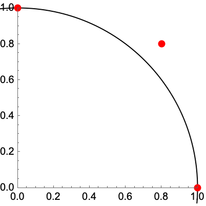
By default, "Criteria"->"Magnitude" selects a largest-magnitude eigenpair:
Eigensystem[m, 1, Method -> "Arnoldi"]Find the largest real-part eigenpair:
Eigensystem[m, 1, Method -> {"Arnoldi", "Criteria" -> "RealPart"}]Find the largest imaginary-part eigenpair:
Eigensystem[m, 1, Method -> {"Arnoldi", "Criteria" -> "ImaginaryPart"}]Find two eigenpairs from both ends of the symmetric matrix spectrum:
d = DiagonalMatrix[{1, 0.8, -1, 2}];
t = Orthogonalize[{{1, 2, 0, 1}, {0, 3, 2, -2}, {1, 0, 4, -1}, {0, 1, 0, 1}}];
m = t.d.Transpose[t];Eigensystem[m, 2, Method -> {"Arnoldi", "Criteria" -> "BothEnds"}]Use "StartingVector" to avoid randomness:
d = DiagonalMatrix[{1, -1, 0.}];
t = {{1, 2, 0}, {0, 3, 2}, {1, 0, 4}};
m = t.d.Inverse[t];
Different starting vectors may converge to different eigenpairs:
Eigensystem[m, 1, Method -> {"Arnoldi", "StartingVector" -> {1, 0, 0}}]Eigensystem[m, 1, Method -> {"Arnoldi", "StartingVector" -> {0, 0, 1}}]Use "Shift"->μ to shift the eigenvalues by transforming the matrix ![]() to
to ![]() . This preserves the eigenvectors but changes the eigenvalues by -μ. The method compensates for the changed eigenvalues. "Shift" is typically used to find eigenpairs when there are no criteria such as largest or smallest magnitude that can select them:
. This preserves the eigenvectors but changes the eigenvalues by -μ. The method compensates for the changed eigenvalues. "Shift" is typically used to find eigenpairs when there are no criteria such as largest or smallest magnitude that can select them:
d = DiagonalMatrix[{1, 2, 3}];
t = {{1, 2, 0}, {0, 3, 2}, {1, 0, 4}};
m = N@t.d.Inverse[t];μ = 2.1;Manually shift the matrix and adjust the resulting eigenvalue:
{λl1, vl1} = Eigensystem[m - μ IdentityMatrix[3], -1, Method -> "Arnoldi"]λl1 = λl1 + μAutomatically shift and adjust the eigenvalue:
{λl2, vl2} = Eigensystem[m, -1, Method -> {"Arnoldi", "Shift" -> μ}]Compute two smallest generalized eigenvalues and eigenvectors with the Arnoldi method:
n = 10;
s = SparseArray[{{i_, i_} -> -2., {i_, j_} /; Abs[i - j] == 1 -> 1.}, {n, n}];
m = SparseArray[{{i_, i_} -> 1}, {n, n}];
Eigensystem[{s, m}, -2, Method -> "Arnoldi"]
"Banded" (1)
The banded method can be used for real symmetric or complex Hermitian machine-precision matrices. The method is most useful for finding all eigenpairs.
Compute the two largest eigenpairs for a banded matrix:
m = SparseArray[{{i_, i_} -> -2., {i_, j_} /; Abs[i - j] == 1 -> 1.}, {2000, 2000}];MatrixPlot[m]{λl, vl} = Eigensystem[m, 2, Method -> "Banded"];λlNorm[m.Transpose[vl] - Transpose[vl].DiagonalMatrix[λl]]"FEAST" (2)
The FEAST method can be used for real symmetric or complex Hermitian machine-precision matrices. The method is most useful for finding eigenvalues in a given interval.
The following suboptions can be specified for the method "FEAST":
| "ContourPoints" | select the number of contour points | |
| "Interval" | an interval for finding eigenvalues | |
| "MaxIterations" | the maximum number of refinement loops | |
| "NumberOfRestarts" | the maximum number of restarts | |
| "SubspaceSize" | the initial size of subspace | |
| "Tolerance" | the tolerance to terminate refinement | |
| "UseBandedSolver" | whether to use a banded solver |
Compute eigenpairs in the interval ![]() :
:
s = SparseArray[{{i_, i_} -> -2., {i_, j_} /; Abs[i - j] == 1 -> 1.}, {1000, 1000}];Use "Interval" to specify the interval:
{λl, vl} = Eigensystem[s, Method -> {"FEAST", "Interval" -> {-1.0, -0.9}}]; λlThe interval end points ![]() are not included in the interval FEAST finds eigenvalues in.
are not included in the interval FEAST finds eigenvalues in.
Norm[s.Transpose[vl] - Transpose[vl].DiagonalMatrix[λl]]Quartics (1)
m = Table[{1, 2, -1, -2} ^ j, {j, 4}]In general, for a 4×4 matrix, the result will be given in terms of Root objects:
Eigensystem[m]You can get the result in terms of radicals using the Cubics and Quartics options:
Short[Eigensystem[m, Cubics -> True, Quartics -> True], 10]Applications (16)
The Geometry of Eigensystem (3)
Eigenvectors with positive eigenvalues point in the same direction when acted on by the matrix:
m = {{1, 2}, {2, 1}};
{{λ1, λ2}, {v1, v2}} = Eigensystem[m]Graphics[{{Thick, Arrow[{{0, 0}, v1}]}, {Red, Arrow[{{0, 0}, m.v1}]}}, Axes -> True]Eigenvectors with negative eigenvalues point in the opposite direction when acted on by the matrix:
Graphics[{{Thick, Arrow[{{0, 0}, v2}]}, {Red, Arrow[{{0, 0}, m.v2}]}}, Axes -> True]Consider the following matrix ![]() and its associated quadratic form
and its associated quadratic form ![]() :
:
a = {{-2, 2}, {2, 1}};q = {x, y}.a.{x, y}//ExpandThe eigenvectors are the axes of the hyperbolas defined by ![]() :
:
{λ, v} = Eigensystem[a]The sign of the eigenvalue corresponds to the sign of the right-hand side of the hyperbola equation:
ContourPlot[Table[q == n, {n, {-9, -4, -1, 1, 4, 9}}]//Evaluate, {x, -3, 3}, {y, -3, 3}, Epilog -> (Arrow[{{0, 0}, #}]& /@ v), PlotLegends -> "Expressions"]Here is a positive-definite quadratic form in 3 dimensions:
q = 20 x ^ 2 - 16 x y + 23 y ^ 2 - 12 x z - 2 y z + 17 z ^ 2;cp = ContourPlot3D[q, {x, -1, 1}, {y, -1, 1}, {z, -1, 1}, Contours -> {10}, Mesh -> False, ContourStyle -> Opacity[.5]]Get the symmetric matrix for the quadratic form, using CoefficientArrays:
m = Normal[CoefficientArrays[q, {x, y, z}, Symmetric -> True][[3]]]Numerically compute its eigenvalues and eigenvectors:
{vals, vecs} = Eigensystem[N[m]]Show the principal axes of the ellipsoid:
Show[cp, Graphics3D[{Thickness[0.015], Green, Table[Line[{{0, 0, 0}, vecs[[i]] * Sqrt[10 / vals[[i]]]}], {i, 1, 3}]}]]Diagonalization (5)
Diagonalize the following matrix as ![]() . First, compute
. First, compute ![]() 's eigenvalues and eigenvectors:
's eigenvalues and eigenvectors:
m = {{9, -7, 3}, {12, -10, 3}, {16, -16, 1}};Eigensystem[m]Construct a diagonal matrix ![]() from the eigenvalues and a matrix
from the eigenvalues and a matrix ![]() whose columns are the eigenvectors:
whose columns are the eigenvectors:
{d = DiagonalMatrix[First[%]], p = Transpose[Last[%]]}m == p.d.Inverse[p]Any function of the matrix can now be computed as ![]() . For example, MatrixPower:
. For example, MatrixPower:
MatrixPower[m, k] == p . MatrixPower[d, k].Inverse[p]Similarly, MatrixExp becomes trivial, requiring only exponentiating the diagonal elements of ![]() :
:
MatrixExp[m] == p . MatrixExp[d].Inverse[p]MatrixExp[d]Let ![]() be the linear transformation whose standard matrix is given by the matrix
be the linear transformation whose standard matrix is given by the matrix ![]() . Find a basis
. Find a basis ![]() for
for ![]() with the property that the representation of
with the property that the representation of ![]() in that basis
in that basis ![]() is diagonal:
is diagonal:
a = (|    |    |   |   |
| -- | -- | - | - |
| -6 | 4  | 0 | 9 |
| -3 | 0  | 1 | 6 |
| -1 | -2 | 1 | 0 |
| -4 | 4  | 0 | 7 |);
Find the eigenvalues and eigenvectors of ![]() :
:
{λ, v} = Eigensystem[a]Let ![]() consist of the eigenvectors, and let
consist of the eigenvectors, and let ![]() be the matrix whose columns are the elements of
be the matrix whose columns are the elements of ![]() :
:
b = Transpose[v]![]() converts from
converts from ![]() -coordinates to standard coordinates. Its inverse converts in the reverse direction:
-coordinates to standard coordinates. Its inverse converts in the reverse direction:
bInv = Inverse[b]Thus ![]() is given by
is given by ![]() , which is diagonal:
, which is diagonal:
bInv . a .b//MatrixFormNote that this is simply the diagonal matrix whose entries are the eigenvalues:
% == DiagonalMatrix[λ]A real-valued symmetric matrix is orthogonally diagonalizable as ![]() , with
, with ![]() diagonal and real valued and
diagonal and real valued and ![]() orthogonal. Verify that the following matrix is symmetric and then diagonalize it:
orthogonal. Verify that the following matrix is symmetric and then diagonalize it:
(s = {{1, 4, -2}, {4, 5, -3}, {-2, -3, 2}})//MatrixFormTranspose[s] == sCompute the eigenvalues and eigenvectors:
{λ, v} = Eigensystem[s]The matrix ![]() has the eigenvalues on the diagonal:
has the eigenvalues on the diagonal:
d = DiagonalMatrix[λ]For an orthogonal matrix, it is necessary to normalize the eigenvectors before placing them in columns:
o = Transpose[FullSimplify[Normalize /@ v]]OrthogonalMatrixQ[o]s == o.d.Transpose[o]//FullSimplifyA matrix is called normal if ![]() . Normal matrices are the most general kind of matrix that can be diagonalized by a unitary transformation. All real symmetric matrices
. Normal matrices are the most general kind of matrix that can be diagonalized by a unitary transformation. All real symmetric matrices ![]() are normal because both sides of the equality are simply
are normal because both sides of the equality are simply ![]() :
:
TensorExpand[ConjugateTranspose[s].s == s.ConjugateTranspose[s] == s.s, Assumptions -> s∈Matrices[{n, n}, Reals, Symmetric[{1, 2}]]]Show that the following matrix is normal, then diagonalize it:
(n = {{3, -1}, {1, 3}})//MatrixFormn.ConjugateTranspose[n] == ConjugateTranspose[n].nConfirm using NormalMatrixQ:
NormalMatrixQ[n]Find the eigenvalues and eigenvectors:
{λ, v} = Eigensystem[n]Unlike a real symmetric matrix, the diagonal matrix for this matrix is complex valued:
(d = DiagonalMatrix[λ])//MatrixFormNormalizing the eigenvectors and putting them in columns gives a unitary matrix:
u = Transpose[Normalize /@ v];
UnitaryMatrixQ[u]n == u.d.ConjugateTranspose[u]The eigensystem of a nondiagonalizable matrix:
m = {{1, 1, 0}, {0, 1, 0}, {0, 0, 2}};
{λ, vecs} = Eigensystem[m]
The dimension of the span of all the eigenvectors is less than the number of eigenvalues:
Count[vecs, v_ /; Norm[v] > 0] < Length[λ]Estimate the probability that a random 4×4 matrix of ones and zeros is not diagonalizable:
Block[{nd = 0, trials = 10 ^ 4}, Do[{λ, vecs} = Eigensystem[N[RandomInteger[1, {4, 4}]]];If[Count[vecs, v_ /; Norm[v] > 0] < Length[λ], nd++], {trials}];N[nd / trials]]Differential Equations and Dynamical Systems (4)
Solve the system of ODEs ![]() ,
, ![]() ,
, ![]() . First, construct the coefficient matrix
. First, construct the coefficient matrix ![]() for the right-hand side:
for the right-hand side:
a = {{0, 1, 0}, {0, 0, 1}, {-2, 1, 2}};Find the eigenvalues and eigenvectors:
{λ, v} = Eigensystem[a]Construct a diagonal matrix whose entries are the exponential of ![]() :
:
d = DiagonalMatrix[Exp[t λ]]Construct the matrix whose columns are the corresponding eigenvectors:
p = Transpose[v]The general solution is ![]() , for three arbitrary starting values:
, for three arbitrary starting values:
p.d.Inverse[p] . {C[1], C[2], C[3]}Verify the solution using DSolveValue:
Simplify[% == DSolveValue[{x'[t] == y[t], y'[t] == z[t], z'[t] == -2x[t] + y[t] + 2z[t]}, {x[t], y[t], z[t]}, t]]Suppose a particle is moving in a planar force field and its position vector ![]() satisfies
satisfies ![]() and
and ![]() , where
, where ![]() and
and ![]() are as follows. Solve this initial problem for
are as follows. Solve this initial problem for ![]() :
:
a = (|    |    |
| -- | -- |
| 4  | -5 |
| -2 | 1 |);Subscript[x, 0] = (| |
| --- |
| 1.9 |
| 3.6 |);First, compute the eigenvalues and corresponding eigenvectors of ![]() :
:
{λ, v} = Eigensystem[a]The general solution of the system is ![]() . Use LinearSolve to determine the coefficients:
. Use LinearSolve to determine the coefficients:
c = LinearSolve[Transpose[v], Subscript[x, 0]]Construct the appropriate linear combination of the eigenvectors:
x[t_] = (c Exp[λ t]).vVerify the solution using DSolveValue:
x[t] == DSolveValue[{{u1'[t], u2'[t]} == a.{u1[t], u2[t]}, {u1[0], u2[0]} == Subscript[x, 0]}, {u1[t], u2[t]}, t] //Simplify//ChopProduce the general solution of the dynamical system ![]() when
when ![]() is the following stochastic matrix:
is the following stochastic matrix:
a = (|     |     |     |
| --- | --- | --- |
| .90 | .01 | .09 |
| .01 | .90 | .01 |
| .09 | .09 | .90 |);
Find the eigenvalues and eigenvectors, using Chop to discard small numerical errors:
{{Subscript[λ, 1], Subscript[λ, 2], Subscript[λ, 3]}, {Subscript[v, 1], Subscript[v, 2], Subscript[v, 3]}} = Chop[Eigensystem[a]]The general solution is an arbitrary linear combination of terms of the form ![]() :
:
x[k_] = Sum[C[i] Subsuperscript[λ, i, k]Subscript[v, i], {i, 3}]Verify that ![]() satisfies the dynamical equation up to numerical rounding:
satisfies the dynamical equation up to numerical rounding:
x[k] == a.x[k - 1]//Simplify//Chopleqn = {Derivative[1][x][t] == -3(x[t] - y[t]), Derivative[1][y][t] == -x[t] z[t] + 26 x[t] - y[t], Derivative[1][z][t] == x[t] y[t] - z[t]};Find the Jacobian for the right-hand side of the equations:
lj = D[leqn[[All, 2]], {{x[t], y[t], z[t]}}]eqp = Solve[leqn /. {x'[t] -> 0, y'[t] -> 0, z'[t] -> 0}, {x[t], y[t], z[t]}]Find the eigenvalues and eigenvectors of the Jacobian at the equilibrium point in the first octant:
{vals, vecs} = Eigensystem[N[lj /. eqp[[3]]]]A function that integrates backward from a small perturbation of pt in the direction dir:
st[pt_, dir_] := First[{x[t], y[t], z[t]} /. NDSolve[{leqn, Thread[{x[0], y[0], z[0]} == pt + 10^-6dir]}, {x, y, z}, {t, 0, -4}]];Show the stable curve for the equilibrium point on the right:
pt = {x[t], y[t], z[t]} /. eqp[[3]];dir = vecs[[3]];sr = ParametricPlot3D[Evaluate[{st[pt, dir], st[pt, -dir]}], {t, 0, -4}, PlotStyle -> Table[{Thickness[0.015], Red}, {2}]]Find the stable curve for the equilibrium point on the left:
pt = {x[t], y[t], z[t]} /. eqp[[2]];{vals, vecs} = Eigensystem[N[lj /. eqp[[2]]]];
dir = vecs[[3]];sl = ParametricPlot3D[Evaluate[{st[pt, dir], st[pt, -dir]}], {t, 0, -4}, PlotStyle -> Table[{Thickness[0.015], Green}, {2}]];
Show the stable curves along with a solution of the Lorenz equations:
Show[{ParametricPlot3D[Evaluate[{x[t], y[t], z[t]} /. NDSolve[{leqn, x[0] == 5, y[0] == 0, z[0] == 25}, {x, y, z}, {t, 0, 100}]], {t, 0, 100}], sr, sl}, PlotRange -> {{-25, 25}, {-25, 25}, {0, 50}}]Physics (4)
In quantum mechanics, states are represented by complex unit vectors and physical quantities by Hermitian linear operators. The eigenvalues represent possible observations and the squared modulus of the components with respect to eigenvectors the probabilities of those observations. For the spin operator ![]() and state
and state ![]() given, find the possible observations and their probabilities:
given, find the possible observations and their probabilities:
σ = (ℏ/2)(| | |
| - | -- |
| 0 | -I |
| I | 0 |);ψ = (1/Sqrt[5])(| |
| --- |
| 1 |
| 2 I |);Computing the eigensystem, the possible observations are ![]() :
:
{λ, v} = Eigensystem[σ]Normalize the eigenvectors in order to compute proper projections:
{e1, e2} = Normalize /@ vThe relative probabilities are ![]() for
for ![]() and
and ![]() for
for ![]() :
:
{Abs[e1.ψ]^2, Abs[e2.ψ]^2}//SimplifyIn quantum mechanics, the energy operator is called the Hamiltonian ![]() , and a state with energy
, and a state with energy ![]() evolves according to the Schrödinger equation
evolves according to the Schrödinger equation ![]() . Given the Hamiltonian for a spin-1 particle in constant magnetic field in the
. Given the Hamiltonian for a spin-1 particle in constant magnetic field in the ![]() direction, find the state at time
direction, find the state at time ![]() of a particle that is initially in the state
of a particle that is initially in the state ![]() representing
representing ![]() :
:
ℋ = (Subscript[ω, 0]ℏ/Sqrt[2]) (|   |    |    |
| - | -- | -- |
| 0 | -I | 0  |
| I | 0  | -I |
| 0 | I  | 0  |);Subscript[ψ, 0] = {1, 0, 0};
Computing the eigensystem, the energy levels are ![]() and
and ![]() :
:
{{Subscript[ℰ, 1], Subscript[ℰ, 2], Subscript[ℰ, 3]}, v} = Eigensystem[ℋ]{Subscript[e, 1], Subscript[e, 2], Subscript[e, 3]} = Normalize /@ vThe state at time ![]() is the sum of each eigenstate evolving according to the Schrödinger equation:
is the sum of each eigenstate evolving according to the Schrödinger equation:
ψ[t_] = Underoverscript[∑, i = 1, 3]Exp[-(I Subscript[ℰ, i]t/ℏ)]Subscript[e, i].Subscript[ψ, 0] Subscript[e, i] //FullSimplifyThe moment of inertia is a real symmetric matrix that describes the resistance of a rigid body to rotating in different directions. The eigenvalues of this matrix are called the principal moments of inertia, and the corresponding eigenvectors (which are necessarily orthogonal) the principal axes. Find the principal moments of inertia and principal axes for the following tetrahedron:
tet = Tetrahedron[{{-1.25, -1, -0.75}, {3.75, -1, -0.75}, {-1.25, 3., -0.75}, {-1.25, -1, 2.25}}]First compute the moment of inertia:
(ℐ = MomentOfInertia[tet])//MatrixFormCompute the principal moments and axes:
{m, a} = Eigensystem[ℐ]Verify that the axes are orthogonal:
a.a//ChopThe center of mass of the tetrahedron is at the origin:
RegionCentroid[tet]Visualize the tetrahedron and its principal axes:
Graphics3D[{{Opacity[.5], tet}, Arrow[{{0, 0, 0}, 3#}]& /@ a}]A generalized eigensystem can be used to find normal modes of coupled oscillations that decouple the terms. Consider the system shown in the diagram:
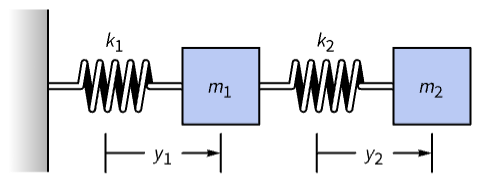
By Hooke's law it obeys ![]() ,
, ![]() . Substituting in the generic solution
. Substituting in the generic solution ![]() gives rise to the matrix equation
gives rise to the matrix equation ![]() , with the stiffness matrix
, with the stiffness matrix ![]() and mass matrix
and mass matrix ![]() as follows:
as follows:
k = {{k1 + k2, -k2}, {-k2, k2}};
m = {{m1, 0}, {0, m2}};
Find the eigenfrequencies and normal modes if ![]() ,
, ![]() ,
, ![]() and
and ![]() :
:
k = k /. {k1 -> 9.5, k2 -> 4.5};
m = m /. {m1 -> 2, m2 -> 3};
Solve the generalized eigenvalue value problem:
{λ, v} = Eigensystem[{k, m}]The eigenfrequencies ![]() are the square roots of the eigenvalues:
are the square roots of the eigenvalues:
{ω1, ω2} = Sqrt[λ]Construct the normal mode solutions as a generalized eigenvector times the corresponding exponential:
sol1[t_] = First[v]Exp[I ω1 t];sol2[t_] = Last[v]Exp[I ω2 t];Verify that both satisfy the differential equation for the system:
-k.sol1[t] == m.sol1''[t] && -k.sol2[t] == m.sol2''[t]//FullSimplifyProperties & Relations (17)
The eigenvectors returned for a numerical matrix are unit vectors:
{λ, v} = Eigensystem[{{1., 2.}, {2., 1.}}]Norm /@ vThe eigenvectors returned for exact and symbolic matrices are typically not unit vectors:
{λ, v} = Eigensystem[{{1, 2}, {2, 1}}]Norm /@ vEigensystem[m] is effectively equivalent to {Eigenvalues[m],Eigenvectors[m]}:
m = RandomReal[1, {3, 3}];
Eigensystem[m] == {Eigenvalues[m], Eigenvectors[m]}
If both eigenvectors and eigenvalues are needed, it is generally more efficient to just call Eigensystem:
m = RandomReal[1, {1000, 1000}];AbsoluteTiming[Eigensystem[m];]AbsoluteTiming[{Eigenvalues[m], Eigenvectors[m]};]Any square matrix satisfies its similarity relation:
m = {{1, 2, 3}, {4, 5, 6}, {7, 8, 9}};
{vals, vecs} = Eigensystem[m];Simplify[m.Transpose[vecs] - Transpose[vecs].DiagonalMatrix[vals]]Any pair of square matrices satisfies the generalized similarity relation for finite eigenvalues:
m = {{1, 2, 3}, {4, 5, 6}, {7, 8, 9}};
a = {{1, 1, 1}, {1, 2, 4}, {1, 3, 9}};
{gvals, gvecs} = Eigensystem[{m, a}];m.Transpose[gvecs] - a.Transpose[gvecs].DiagonalMatrix[gvals]//SimplifyAn infinite generalized eigenvalue of ![]() corresponds to an eigenvector of
corresponds to an eigenvector of ![]() that is in the kernel of
that is in the kernel of ![]() :
:
m = {{1, 2}, {3, 2}};
a = {{1, 1}, {1, 1}};
Eigensystem[{m, a}]
The vector ![]() is an eigenvector of
is an eigenvector of ![]() with eigenvalue
with eigenvalue ![]() :
:
m.{-1, 1}It is also in the null space of ![]() :
:
a.{-1, 1}A matrix m has a complete set of eigenvectors iff DiagonalizableMatrixQ[m] is True:
diag = {{17, -1 + Sqrt[3], -1 - Sqrt[3]}, {-1 + Sqrt[3], 14 + 2 Sqrt[3], 2}, {-1 - Sqrt[3], 2, 14 - 2 Sqrt[3]}};
{DiagonalizableMatrixQ[diag], Eigensystem[diag]}
The following matrix is missing an eigenvector for the space ![]() , symbolized by
, symbolized by ![]() :
:
nondiag = {{15, 3 + 3 Sqrt[3], 0}, {0, 15 + 3 Sqrt[3], 3}, {3 - 3 Sqrt[3], 0, 15 - 3 Sqrt[3]}};
{DiagonalizableMatrixQ[nondiag], Eigensystem[nondiag]}
For a diagonalizable matrix, Eigensystem reduces function application to application to eigenvalues:
m = N[{{0, 1, 0, -1}, {-1, 0, 1, 0}, {0, -1, 0, 1}, {1, 0, -1, 0}}];
{vals, vecs} = Eigensystem[m];
Compute the matrix exponential using diagonalization:
Chop[Transpose[vecs].DiagonalMatrix[Exp[vals]].Inverse[Transpose[vecs]]]Compute the matrix exponential using MatrixExp:
MatrixExp[m]Note that this is not simply the exponential of each entry:
Exp[m]For an invertible matrix ![]() ,
, ![]() and
and ![]() have the same eigenvectors and reciprocal eigenvalues:
have the same eigenvectors and reciprocal eigenvalues:
m = {{0, 3, 7}, {0, -3, 1}, {-4, 2, -8}};
{λ, v} = Eigensystem[m]
Because eigenvalues are sorted by absolute value, this gives the same values but in the opposite order:
{λInv, vInv} = Eigensystem[Inverse[m]];
{(1/λInv), vInv}//FullSimplify
For an analytic function ![]() , the eigenvectors of
, the eigenvectors of ![]() are also eigenvectors of
are also eigenvectors of ![]() with eigenvalue
with eigenvalue ![]() :
:
m = {{1, 1, 0}, {-1, 1, 0}, {0, 0, 5}};
{λ, v} = Eigensystem[m]
For example, the ![]() has the same eigenvectors with squared eigenvalues:
has the same eigenvectors with squared eigenvalues:
Eigensystem[m.m] == {λ^2, v}Similarly, the eigenvalues of ![]() are
are ![]() :
:
Eigensystem[MatrixExp[m]] == {Exp[λ], v}//FullSimplifyThe eigenvalues of a real symmetric matrix are real and its eigenvectors are orthogonal:
(s = {{1, 4, -2}, {4, 0, -3}, {-2, -3, 2}})//MatrixFormSymmetricMatrixQ[s]By inspection, the eigenvalues are real:
{λ, v} = Eigensystem[s]Confirm the eigenvectors are orthogonal to each other:
v.Transpose[v]//SimplifyThe eigenvalues of a real antisymmetric matrix are imaginary and its eigenvectors are orthogonal:
(a = {{0, 4, -2}, {-4, 0, -3}, {2, 3, 0}})//MatrixFormAntisymmetricMatrixQ[a]By inspection, the eigenvalues are imaginary:
{λ, v} = Eigensystem[a]Confirm the eigenvectors are orthogonal to each other:
v.ConjugateTranspose[v]//SimplifyThe eigenvalues of a unitary matrix lie on the unit circle and its eigenvectors are orthogonal:
u = {{1 / Sqrt[2], I / Sqrt[2]}, {I / Sqrt[2], 1 / Sqrt[2]}};UnitaryMatrixQ[u]Compute the eigenvalues and eigenvectors:
{λ, v} = Eigensystem[u]Confirm that the eigenvalues lie on the unit circle:
Abs[λ]Confirm the eigenvectors are orthogonal to each other:
v.ConjugateTranspose[v]//SimplifyThe eigenvectors of any normal matrix are orthogonal:
n = {{1, 2, -1}, {-1, 1, 2}, {2, -1, 1}};NormalMatrixQ[n]The eigenvalues can be arbitrary:
{λ, v} = Eigensystem[n]But the eigenvectors are orthogonal:
v.ConjugateTranspose[v]//SimplifySingularValueDecomposition[m] is built from the eigensystems of ![]() and
and ![]() :
:
m = (| | | |
| ---- | --- | ---- |
| -5.2 | 0 | -5 |
| 1.7 | 5.4 | -4.3 |);{u, Σ, v} = SingularValueDecomposition[m];{Subscript[λ, L], Subscript[vec, L]} = Eigensystem[m . ConjugateTranspose[m]];The columns of ![]() are the eigenvectors:
are the eigenvectors:
{u//MatrixForm, Transpose[Subscript[vec, L]]//MatrixForm}{Subscript[λ, R], Subscript[vec, R]} = Eigensystem[ConjugateTranspose[m].m];The columns of ![]() are the eigenvectors:
are the eigenvectors:
{v//MatrixForm, Transpose[Subscript[vec, R]]//MatrixForm}Since ![]() has fewer rows than columns, the diagonal entries of
has fewer rows than columns, the diagonal entries of ![]() are
are ![]() :
:
{Diagonal[Σ], Sqrt[Subscript[λ, L]]}Consider a matrix ![]() with a complete set of eigenvectors:
with a complete set of eigenvectors:
m = {{-(1/Sqrt[2]), -(1/Sqrt[2])}, {(1/Sqrt[2]), -(1/Sqrt[2])}};
{λ, v} = Eigensystem[m]JordanDecomposition[m] returns matrices ![]() built from eigenvalues and eigenvectors:
built from eigenvalues and eigenvectors:
{s, j} = JordanDecomposition[m]The ![]() matrix is diagonal with the eigenvalues as entries:
matrix is diagonal with the eigenvalues as entries:
j == DiagonalMatrix[λ]The ![]() matrix has the corresponding eigenvectors as its columns:
matrix has the corresponding eigenvectors as its columns:
s == Transpose[v]SchurDecomposition[n,RealBlockDiagonalFormFalse] for a numerical normal matrix ![]() :
:
n = {{1., 3., -1.}, {-1., 1., 3.}, {3., -1., 1.}};
NormalMatrixQ[n]{q, t} = SchurDecomposition[n, RealBlockDiagonalForm -> False]//ChopThe matrices {q,t} are built from eigenvalues and eigenvectors:
{λ, v} = Eigensystem[n]//ChopThe t matrix is diagonal and with eigenvalue entries, possibly in a different order from Eigensystem:
Diagonal[t] == λTo verify that q has eigenvectors as columns, set the first entry of each vector to 1. to eliminate phase differences between q and v:
Transpose[(#1/First[q])& /@ q] - (v / First /@ v)//ChopIf matrices share a dimension‐![]() null space,
null space, ![]() of their generalized eigenvalues will be Indeterminate and the eigenvector list will be padded with zeros:
of their generalized eigenvalues will be Indeterminate and the eigenvector list will be padded with zeros:
a = {{1, 1, 1}, {1, 1, 1}, {1, 1, 1}};b = {{1, 2, 3}, {4, 5, 6}, {7, 8, 9}};NullSpace[a]Two generalized eigenvalues of ![]() are Indeterminate and produce zero vectors:
are Indeterminate and produce zero vectors:
Eigensystem[{a, a}]The matrix ![]() has a one-dimensional null space:
has a one-dimensional null space:
NullSpace[b]It lies in the null space of ![]() :
:
MatrixRank[Join[NullSpace[a], NullSpace[b]]]Thus, one generalized eigenvalue of ![]() is Indeterminate and produces a zero vector:
is Indeterminate and produces a zero vector:
Eigensystem[{a, b}]Possible Issues (5)
The general symbolic case very quickly gets very complicated:
Array[Subscript[a, ##]&, {2, 2}]Eigensystem[%]The expression sizes increase faster than exponentially:
Table[ByteCount[Eigensystem[Array[Subscript[a, ##]&, {n, n}]]], {n, 4}]Not all matrices have a complete set of eigenvectors:
Eigensystem[{{7, -1}, {9, 1}}]Use JordanDecomposition for exact computation:
JordanDecomposition[{{7, -1}, {9, 1}}]Use SchurDecomposition for numeric computation:
SchurDecomposition[N@{{7, -1}, {9, 1}}]Construct a 10,000×10,000 sparse matrix:
n = 10^4;s = SparseArray[{Band[{1, 1}] -> 1., Band[{1, -1}, {-1, 1}, {1, -1}] -> 1., Band[{n / 2, 1}, {1, -1}, {0, 1}] -> 1., Band[{1, n / 2}, {-1, 1}, {1, 0}] -> 1.}, {n, n}];ArrayPlot[s, MaxPlotPoints -> 1000, ColorFunction -> (If[# == 0, White, Black]&)]The eigenvector matrix is a dense matrix and too large to represent:
MemoryConstrained[Eigensystem[s], 10 ^ 8]Computing the few largest or smallest eigenvalues is usually possible:
{vals, vecs} = Eigensystem[s, 2]; valsWhen eigenvalues are closely grouped the iterative method for sparse matrices may not converge:
s = SparseArray[{{x_, y_} /; Abs[x - y] ≤ 1 -> 3. Abs[x - y] - 2.}, {1000, 1000}];The iteration has not converged well after 1000 iterations:
{vals, vecs} = Eigensystem[s, 3];
ListPlot[vecs, PlotLabel -> vals]
You can give the algorithm a shift near the expected value to speed up convergence:
{vals, vecs} = Eigensystem[s, 3, Method -> {"Arnoldi", "Shift" -> -4}];ListPlot[vecs, PlotLabel -> vals]The end points given to an interval as specified for the FEAST method are not included.
Set up a matrix with eigenvalues at 3 and 9 and find the eigenvalues and eigenvectors in the interval ![]() :
:
ck = With[{n = 24}, N[SparseArray[{{i_, j_} /; Abs[i - j] == 1 :> With[{k = Min[i, j]}, Sqrt[k (n - k)]]}, {n, n}]]];
{vals, vecs} = Eigensystem[ck, Method -> {"FEAST", "Interval" -> {3., 9.}}];
vals
Enlarge the to interval ![]() such that FEAST finds the eigenvalues 3 and 9 and their corresponding eigenvectors:
such that FEAST finds the eigenvalues 3 and 9 and their corresponding eigenvectors:
{vals, vecs} = Eigensystem[ck, Method -> {"FEAST", "Interval" -> {2.9, 9.1}}];
valsText
Wolfram Research (1988), Eigensystem, Wolfram Language function, https://reference.wolfram.com/language/ref/Eigensystem.html (updated 2024).
CMS
Wolfram Language. 1988. "Eigensystem." Wolfram Language & System Documentation Center. Wolfram Research. Last Modified 2024. https://reference.wolfram.com/language/ref/Eigensystem.html.
APA
Wolfram Language. (1988). Eigensystem. Wolfram Language & System Documentation Center. Retrieved from https://reference.wolfram.com/language/ref/Eigensystem.html