Wolfram言語＆システムドキュメントセンター

SmoothPointDensity

SmoothPointDensity[pdata]

点密度関数を点データ pdata について推定する．

SmoothPointDensity[pdata,bw]

点データ pdata についての密度を帯域幅 bw で推定する．

SmoothPointDensity[pdata,bw,ker]

点データ pdata についての密度を帯域幅 bw と平滑化カーネル ker で推定する．

SmoothPointDensity[bdata,…]

点データ関数をビン分割データ bdata について推定する．

SmoothPointDensity[pproc,…]

密度関数を点過程pproc について計算する．

SmoothPointDensity

SmoothPointDensity[pdata]

点密度関数を点データ pdata について推定する．

SmoothPointDensity[pdata,bw]

点データ pdata についての密度を帯域幅 bw で推定する．

SmoothPointDensity[pdata,bw,ker]

点データ pdata についての密度を帯域幅 bw と平滑化カーネル ker で推定する．

SmoothPointDensity[bdata,…]

点データ関数をビン分割データ bdata について推定する．

SmoothPointDensity[pproc,…]

密度関数を点過程pproc について計算する．

詳細とオプション

点密度は点強度としても知られている．
SmoothPointDensityは点の数が観測領域の長さ，面積，体積によってどのように変わるかを記述する関数を与える．領域上での積分は点の総数である．

SmoothPointDensityはカーネルに基づく点密度の推定器である．帯域幅 bw とカーネル ker を使って平滑化が制御される．

SmoothPointDensityは，密度関数を繰り返し評価するために使えるPointDensityFunctionを返す．
点 pdata は次の形式でよい．

	{p₁,p₂,…}	点 p_i
	GeoPosition[…],GeoPositionXYZ[…],…	地理的な点
	SpatialPointData[…]	空間点集合
	{pts,reg}	点集合 pts と観測領域 reg

観測領域 reg は，与えられていない場合はRipleyRassonRegionを使って自動的に計算される．
点過程 pproc は次の形式でよい．
proc 点過程 proc

{proc,reg} 点過程 proc と観測領域 reg
観測領域 reg は，パラメータフリーで全次元の，SpatialObservationRegionQで調べられるような有界領域である．
点過程 pproc については，厳密な式あるいは近似計算法が使われる．
次の帯域幅指定 bw を使うことができる．

	h	使用する帯域幅
	{"Standardized",h}	標準偏差の単位での帯域幅
	{"Adaptive",h,s}	初期帯域幅 h と感度 s で適応的
	Automatic	自動計算された帯域幅
	"name"	名前付きの帯域幅選択法を使う
	{bw_x,bw_y,…}	x, y 等に別々の帯域幅指定

多変量密度については，h は正定対称行列でよい．
適応的帯域幅については，感度 s は，0から1までの実数かAutomaticでなければならない．Automaticが使われた場合は，s はに設定される．ただし，はデータの次元性である．
次は，使用可能な名前付きの帯域幅選択法である．

	"LeastSquaresCrossValidation"	最小二乗相互検証法を使う
	"Oversmooth"	標準ガウシアンの1.08倍の幅
	"Scott"	Scottの規則を使って帯域幅を決定する
	"SheatherJones"	Sheather–Jonesプラグイン推定器を使う
	"Silverman"	Silvermanの規則を使って帯域幅を決定する
	"StandardDeviation"	標準偏差を帯域幅として使う
	"StandardGaussian"	標準的な正規データのための最適帯域幅

デフォルトで，"Silverman"メソッドが使われる．
自動帯域幅計算については，定数配列は単位分散があるとみなされる．
次のカーネル指定 ker が使える．

	"Biweight"
	"Cosine"
	"Epanechnikov"
	"Gaussian"
	"Rectangular"
	"SemiCircle"
	"Triangular"
	"Triweight"
	func

デフォルトで，"Gaussian"カーネルが使われる．
多変量密度については，カーネル関数 ker は{"Product",ker}および{"Radial",ker}をそれぞれ使って積およびラジアルタイプとして指定できる．タイプの指定がなければ積タイプのカーネルが使われる．
密度推定に使われる精度は bw とデータで与えられる最低精度である．
次は，使用可能なオプションである．
Method Automatic 評価に使用するメソッド
Methodの可能な設定は，Automatic，"KernelMixture"，"SmoothKernel"である．
次は，"KernelMixture"メソッドの使用可能なサブオプションである．
MaxMixtureKernels Automatic 使用するカーネルの最大数
次は，"SmoothKernel"メソッドの使用可能なサブオプションである．

InterpolationPoints	Automatic	使用する補間点の初期数
MaxMixtureKernels	Automatic	使用するカーネルの最大数
MaxRecursion	Automatic	許可する再帰的部分分割数
PerformanceGoal	Automatic	速度あるいは品質について最適化する
MaxExtraBandwidths	Automatic	使用するデータを超えた最大帯域幅

例題

すべて開くすべて閉じる

例 (1)

SpatialPointDataを作成する：

Wolfram Language code: spd = RandomPointConfiguration[PoissonPointProcess[500, 2], Rectangle[]]

点をプロットする：

Wolfram Language code: ListPlot[spd, AspectRatio -> Automatic]

点密度を推定する：

Wolfram Language code: μ = SmoothPointDensity[spd]

点における値：

Wolfram Language code: μ[{.3, .5}]

密度推定を可視化する：

Wolfram Language code: Show[ContourPlot[μ[{x, y}], {x, 0, 1}, {y, 0, 1}], ListPlot[spd, PlotStyle -> Black]]

スコープ (4)

一変量同次SpatialPointDataを作成する：

Wolfram Language code:

reg = Interval[{-3, 3}];
SeedRandom[3];
data = SpatialPointData@RandomPoint[reg, 100]

カーネル混合を使って点密度関数を計算する：

Wolfram Language code: μ = SmoothPointDensity[data, Method -> "KernelMixture"]

タイプを確認する：

Wolfram Language code: μ["Type"]

可視化する：

Wolfram Language code: Plot[μ[{x}], {x, -5, 5}, Filling -> Axis]

一変量非同次SpatialPointDataを作成する：

Wolfram Language code:

reg = Interval[{-3, 3}];
SeedRandom["spatial"];
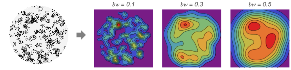
data = RandomPointConfiguration[InhomogeneousPoissonPointProcess[Function[{x}, 1 + x ^ 4], 1], reg]

平滑化カーネル密度を計算する：

Wolfram Language code: μ = SmoothPointDensity[data]

タイプを確認する：

Wolfram Language code: μ["Type"]

可視化する：

Wolfram Language code: Plot[μ[{x}], {x, -6, 6}, PlotRange -> {0, 22}, Filling -> Axis]

クラスタデータの平滑化点密度を計算する：

Wolfram Language code: reg = Disk[{0, 0}, 2];data = RandomPointConfiguration[MaternPointProcess[10, 20, .15, 2], reg];

Wolfram Language code: ListPlot[data, AspectRatio -> Automatic]

平滑化点密度をデータから計算する：

Wolfram Language code: μ = SmoothPointDensity[data]

密度関数とデータ点をプロットする：

Wolfram Language code:

Show[ContourPlot[μ[{x, y}], {x, -2, 2}, {y, -2, 2}, ContourStyle -> None, ColorFunction -> "SolarColors"], ListPlot[data, PlotStyle -> Black]]

ハードコア点過程サンプルについての平滑化点密度を計算する：

Wolfram Language code:

reg = Disk[{0, 0}, 3];data = RandomPointConfiguration[HardcorePointProcess[10, r = 0.2, 2], reg, Method -> {Automatic, "LengthOfRun" -> 10 ^ 4}];

Wolfram Language code: ListPlot[data, AspectRatio -> Automatic]

平滑化点密度をさまざまな帯域幅について計算する：

Wolfram Language code:

bw = {.1, .3, .5};
μ = SmoothPointDensity[data, #, Method -> "SmoothKernel"]& /@ bw;

可視化する：

Wolfram Language code:

Table[Show[ContourPlot[μ[[k]][{x, y}], {x, -3, 3}, {y, -3, 3}, PlotLabel -> Row[{"bandwidth = ", bw[[k]]}], ContourStyle -> None, ColorFunction -> "PearlColors"], ListPlot[data, PlotStyle -> Black]], {k, 3}]

オプション (1)

Method (1)

平滑化点密度を計算するメソッドを比較する：

Wolfram Language code: mthds = {"KernelMixture", "SmoothKernel"};

Wolfram Language code: data = RandomPointConfiguration[ThomasPointProcess[20, 20, .2, 2], reg = Rectangle[]]

点をプロットする：

Wolfram Language code: ListPlot[data]

点密度を推定する：

Wolfram Language code: μ = SmoothPointDensity[data, Method -> #]& /@ mthds;

Wolfram Language code:

GraphicsRow@Table[Show[ContourPlot[μ[[i]][{x, y}], {x, 0, 1}, {y, 0, 1}, PlotLabel -> mthds[[i]], ImageSize -> 250], ListPlot[data, PlotStyle -> Black]], {i, Length[mthds]}]

おもしろい例題 (1)

クラスタ点過程の平滑化点密度：

Wolfram Language code:

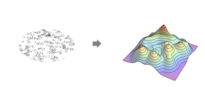
SeedRandom[1];data = RandomPointConfiguration[MaternPointProcess[10, 20, .15, 2], Disk[{0, 0}, 2]];
points = ListPointPlot3D[Map[PadRight[#, 3, 0]&, data["Points"]], PlotStyle -> Gray, Axes -> False, Boxed -> False];
μ = SmoothPointDensity[data];
Show[points, Plot3D[μ[{x, y}], {x, -2, 2}, {y, -2, 2}, PlotRange -> {-200, 500}, Mesh -> None, Axes -> False, Boxed -> False, ColorFunction -> "Rainbow", PlotStyle -> Opacity[.6]], ViewPoint -> {0, 0.00001, 20}]

Top

その他のラーニングリソース

テクニカルサポート

データサイエンス，金融，ビジネス

工学

科学とテクノロジー

教育のためのテクノロジー

教育イニシアチブ

使い始める

Grow Your Skills

Wolframと繋がる

大人用の教育プログラム

若者のための教育プログラム

読む

SmoothPointDensity

詳細とオプション

例題

例 (1)

スコープ (4)

オプション (1)

Method (1)

おもしろい例題 (1)

テキスト

CMS

APA

BibTeX

BibLaTeX

	proc	点過程 proc
	{proc,reg}	点過程 proc と観測領域 reg

SmoothPointDensity

詳細とオプション

例題

例 (1)

スコープ (4)

オプション (1)

Method (1)

おもしろい例題 (1)

関連項目

関連するガイド

履歴

テキスト

CMS

APA

BibTeX

BibLaTeX