TransferFunctionModel
TransferFunctionModel[g[s],s]
represents the model of the transfer-function matrix g[s] with complex variable s.
TransferFunctionModel[{n[s],d[s]},s]
specifies the numerator n[s] and denominator d[s] of a transfer-function model.
TransferFunctionModel[{z,p,g},s]
specifies the zeros z, poles p, and gain g of a transfer-function model.
gives the transfer-function model of the systems model sys.
Details and Options

- TransferFunctionModel is typically used for signal filters and control design.
- A continuous-time system modeled by
 where
where  is the Laplace transform of the output,
  is the Laplace transform of the input and
  is the transfer matrix can be specified as TransferFunctionModel[g[s],s].
 - A discrete-time system modeled by
 where
where  is the Z transform of the output,
  is the Z transform of the input and
  is the transfer matrix can be specified as TransferFunctionModel[g[z],z,SamplingPeriodτ].
 - Time delays can be included in any transfer-function model, by using SystemsModelDelay.
- In TransferFunctionModel[sys], the following systems can be converted:
-
AffineStateSpaceModel approximate Taylor conversion NonlinearStateSpaceModel approximate Taylor conversion StateSpaceModel exact conversion - The following options can be given:
-
Method Automatic the method to obtain the transfer function of a state-space model SamplingPeriod Automatic the sampling period of the system SystemsModelLabels Automatic labels for the input and output variables ExternalTypeSignature Automatic variable types for embedded code - Settings for the Method option include "DeterminantExpansion", "ResolventIdentities", "Inverse", and "Generic". With a setting Method->Automatic, the transfer-function model is computed using determinant expansion.
Examples
open allclose allBasic Examples (5)
Scope (19)
A first-order continuous-time system:
A system with three zeros and six poles:
A first-order discrete-time system:
A two-input, one-output system:
A one-input, two-output system:
A two-input, two-output system:
Specify a transfer function using its numerator and denominator:
A MIMO transfer function specified in terms of its numerators and denominators:
A denominator polynomial that is the least common multiple:
Specify the transfer function, using its algebraic poles, zeros, and gains:
The transfer-function representation of a state-space model:
Taylor linearize an AffineStateSpaceModel and obtain its transfer function representation:
The linearization of an AffineStateSpaceModel with nonzero equilibrium values:
Taylor linearize a NonlinearStateSpaceModel:
Generalizations & Extensions (2)
Options (5)
SamplingPeriod (3)
Applications (18)
A proportional-integral (PI) controller:
A proportional-derivative (PD) controller:
A function to construct a proportional-integral-derivative (PID) controller:
A PID with specific gain values:
A function to construct a discrete-time PID controller:
A function for a continuous-time lead compensator:
A lead compensator for specific values of gain and pole-zero locations:
A function for a continuous-time lag compensator:
A digital lag compensator defined in terms of its zero and pole locations:
A general formula for analog lowpass Butterworth filters:
The general second-order transfer function:
Variations in damping ratio lead to qualitatively different responses:
A linearized inverted pendulum model:

Transfer function between the input voltage and the shaft angular position of a DC motor:
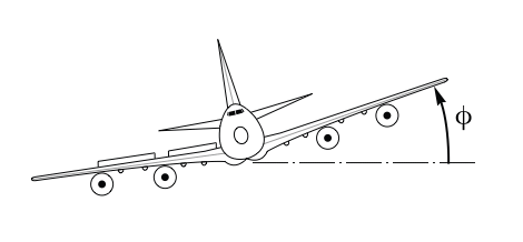
The aileron-to-roll-rate transfer function of an aircraft:

A temperature-controlled chemical reactor:

A MIMO transfer function describing an aircraft's longitudinal dynamics:
A ball mill grinding system with delay due to material transport:
Properties & Relations (8)
TransferFunctionModel behaves as a pure function of one argument:
The value of the transfer-function matrix at a specific frequency:
The values at several frequencies:
Use TransferFunctionFactor to obtain the factored form:
Use TransferFunctionCancel to cancel any common poles and zeros:
Collect terms with similar powers:
Collect terms in any variable:
Find the element zeros and poles of a transfer-function matrix:
Possible Issues (3)
In TransferFunctionModel[m,var], pole-zero pairs may cancel before being processed:
Use Unevaluated to prevent cancellations:
Or use TransferFunctionModel[{num,den},var]:
Or TransferFunctionModel[{z,p,g},var]:
TransferFunctionModel[m,var] might result in a system with higher order:
Or simplify m before passing it to TransferFunctionModel:
If the complex variable var is not specified, it is assumed to be s for continuous-time systems:
Text
Wolfram Research (2010), TransferFunctionModel, Wolfram Language function, https://reference.wolfram.com/language/ref/TransferFunctionModel.html (updated 2014).
CMS
Wolfram Language. 2010. "TransferFunctionModel." Wolfram Language & System Documentation Center. Wolfram Research. Last Modified 2014. https://reference.wolfram.com/language/ref/TransferFunctionModel.html.
APA
Wolfram Language. (2010). TransferFunctionModel. Wolfram Language & System Documentation Center. Retrieved from https://reference.wolfram.com/language/ref/TransferFunctionModel.html