AsymptoticDSolveValue
AsymptoticDSolveValue[eqn,f,xx0]
computes an asymptotic approximation to the differential equation eqn for f[x] centered at x0.
AsymptoticDSolveValue[{eqn1,eqn2,…},{f1,f2,…},xx0]
computes an asymptotic approximation to a system of differential equations.
AsymptoticDSolveValue[eqn,f,x,ϵϵ0]
computes an asymptotic approximation of f[x,ϵ] for the parameter ϵ centered at ϵ0.
AsymptoticDSolveValue[eqn,f,…,{ξ,ξ0,n}]
computes the asymptotic approximation to order n.
Details and Options


- Asymptotic approximations to differential equations are also known as asymptotic expansions, perturbation solutions, regular perturbations and singular perturbations, etc. They are also known by specific methods used to compute some of them, such as Frobenius series, WKB, boundary-layer method, etc.
- Asymptotic approximations are typically used to solve problems for which no exact solution can be found or to get simpler answers for computation, comparison and interpretation.
- AsymptoticDSolveValue[eqn,…,xx0] computes the leading term in an asymptotic expansion for eqn. Use SeriesTermGoal to specify more terms.
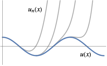
- If the exact result is g[x] and the asymptotic approximation of order n at x0 is gn[x], then the result is AsymptoticLess[g[x]-gn[x],gn[x]-gn-1[x],xx0] or g[x]-gn[x]∈o[gn[x]-gn-1[x]] as xx0.
- The asymptotic approximation gn[x] is often given as a sum gn[x]
 αkϕk[x], where {ϕ1[x],…,ϕn[x]} is an asymptotic scale ϕ1[x]≻ϕ2[x]≻⋯>ϕn[x] as xx0. Then the result is AsymptoticLess[g[x]-gn[x],ϕn[x],xx0] or g[x]-gn[x]∈o[ϕn[x]] as xx0.
 - Common asymptotic scales include:
-

Taylor scale when xx0 
Laurent scale when xx0 
Laurent scale when x±∞ 
Puiseux scale when xx0 - The scales used to express the asymptotic approximation are automatically inferred from the problem and can often include more exotic scales.
- The center x0 can be any finite or infinite real or complex number.
- The order n must be a positive integer and specifies order of approximation for the asymptotic solution. It is not related to polynomial degree.
- The specification u∈Vectors[n] or u∈Matrices[{m,n}] can be used to indicate that the dependent variable u is a vector-valued or a matrix-valued variable, respectively. » »
- The following options can be given:
-
AccuracyGoal Automatic digits of absolute accuracy sought Assumptions $Assumptions assumptions to make about parameters GenerateConditions Automatic whether to generate answers that involve conditions on parameters GeneratedParameters None how to name generated parameters Method Automatic method to use PerformanceGoal $PerformanceGoal aspects of performance to optimize PrecisionGoal Automatic digits of precision sought SeriesTermGoal Automatic number of terms in the approximation WorkingPrecision Automatic the precision used in internal computations - Possible settings for PerformanceGoal include $PerformanceGoal, "Quality" and "Speed". With the "Quality" setting, AsymptoticDSolve typically solves more problems or produces simpler results, but it potentially uses more time and memory.

Examples
open allclose allBasic Examples (3)
Scope (49)
Basic Uses (8)
Compute a series solution of order 10 for an ODE around x=0:
Plot the successive approximations for an asymptotic solution:
Use Accumulate to build the list of approximations:
Compute a series solution around x=3:
Obtain a series approximation for the general solution:
Obtain series approximations with different numbers of terms:
Compute a series solution for a system of ODEs:
Compute a series solution for a perturbation problem:
Ordinary Points (7)
Find a Taylor series solution for a linear first-order ODE at the ordinary point x=0:
Plot the successive approximations given by the solution:
Series solution for a linear second-order ODE at the ordinary point x=0:
Plot the successive approximations given by the solution:
Series solution for an inhomogeneous linear ODE at the ordinary point x=0:
Series solution for a linear ODE with nonrational coefficients at the ordinary point x=0:
Series solution for a linear higher-order ODE at the ordinary point x=0:
Series solution for a linear ODE at the ordinary point x=1:
Series approximation for the general solution for a linear ODE at an ordinary point:
Regular Singular Points (5)
Find a Frobenius series solution for a linear first-order ODE at the regular singular point x=0:
Plot the successive approximations given by the solution:
Series solution for a linear second-order ODE at the regular singular point x=0:
Find a series solution for a linear higher-order ODE at the regular singular point x=0:
The series solution is an exact solution in this case:
Series solution for a linear ODE at the regular singular point x=1:
Series solution for a linear ODE with nonrational coefficients at the regular singular point x=0:
Irregular Singular Points (3)
Find an asymptotic solution for a linear first-order ODE at the irregular singular point x=0:
Plot the successive approximations given by the solution:
Series solution for a linear second-order ODE at the irregular singular point x=0:
Series solution for a linear higher-order ODE at the irregular singular point x=0:
Nonlinear ODEs (7)
Find a series solution for a nonlinear first-order ODE at x=0:
Plot the successive approximations given by the solution:
Series solution for a nonlinear second-order ODE at x=0:
Plot the successive approximations given by the solution:
Series solution for an inhomogeneous nonlinear ODE at the ordinary point x=0:
Series solution for a nonlinear ODE with nonrational coefficients at x=0:
Series solution for a nonlinear higher-order ODE at x=0:
Series solution for a nonlinear ODE at x=1:
Series approximation for the general solution of a nonlinear ODE:
Solutions at Infinity (4)
Systems of ODEs (7)
Find a series solution for a linear system of first-order ODEs at the ordinary point x=0:
Plot the approximation given by the solution:
Series solution for a linear system of higher-order ODEs at the ordinary point x=0:
Series solution for an inhomogeneous system of linear ODEs at the ordinary point x=0:
Series solution for a linear system of ODEs at the ordinary point x=1:
Series approximation to the general solution for a linear system of ODEs at an ordinary point:
Series solution for a linear system of ODEs at the ordinary point x=0 using vector variables:
Series solution for a linear system of ODEs at the ordinary point x=0 using matrix variables:
Regular Perturbations (2)
Singular Perturbations (3)
Find a first-order approximation for a singular boundary value problem:
Plot the approximation for different values of the parameter:
Compare with a numerical solution:
Find a second-order approximation for a singular boundary value problem:
Plot the approximation for different values of the parameter:
Fractional ODEs (3)
Find the series solution for a linear fractional ODE of order 0.7:
Solve the same ODE using DSolveValue:
Compare exact solution with asymptotic solutions for various values of approximation of order ![]() :
:
Find the series solution for a linear fractional ODE with nonconstant coefficients:
Find a series solution for a system of two linear fractional ODEs:
Applications (7)
Compute a Taylor polynomial approximation for Cos:
Improve the range of the approximation by specifying a higher order:
Study the variation of range with the order of the approximation:
Solve Bessel's equation of order ![]() around the regular singular point x=0:
around the regular singular point x=0:
Plot the two components of the general solution:
The Airy equation has an irregular singular point at x=∞:
Compute an asymptotic expansion at the irregular singular point:
Compare with the expansions for the Airy functions at Infinity:
Plot the Airy functions and the approximations:
Compute an exact polynomial solution of a nonlinear first-order ODE:
Verify that this is a solution of the ODE:
Compute an equilibrium solution for a system of first-order ODEs:
Visualize the vector field defined by the system:
Solve the system with general initial conditions:
Find the equilibrium solution:
Find a first-order perturbation expansion for the Duffing equation:
Plot the approximate solution:
Compare with the exact solution:
Find the approximate eigenfunctions for the Sturm–Liouville problem corresponding to ![]() , for large values of
, for large values of ![]() . Rewrite the problem using a small parameter
. Rewrite the problem using a small parameter ![]() :
:
Obtain a first-order asymptotic approximation:
Construct the eigenfunctions after ignoring the constant Csc factor, using ![]() :
:
Properties & Relations (3)
Solutions satisfy the differential equation up to a given order:
Use DSolveValue to find an exact solution:
Use NDSolveValue to find a numerical solution:
Text
Wolfram Research (2018), AsymptoticDSolveValue, Wolfram Language function, https://reference.wolfram.com/language/ref/AsymptoticDSolveValue.html (updated 2022).
CMS
Wolfram Language. 2018. "AsymptoticDSolveValue." Wolfram Language & System Documentation Center. Wolfram Research. Last Modified 2022. https://reference.wolfram.com/language/ref/AsymptoticDSolveValue.html.
APA
Wolfram Language. (2018). AsymptoticDSolveValue. Wolfram Language & System Documentation Center. Retrieved from https://reference.wolfram.com/language/ref/AsymptoticDSolveValue.html