GeometricOptimization[{a0,b0},{{a1,b1},…},{aeq,beq}]
finds the positive vector x=y that minimizes ![]() subject to inequality constraints
subject to inequality constraints ![]() and linear equality constraints
and linear equality constraints ![]() .
.


GeometricOptimization
GeometricOptimization[f,cons,vars]
finds positive values of variables vars that minimize the posynomial objective subject to posynomial constraints cons.
GeometricOptimization[{a0,b0},{{a1,b1},…},{aeq,beq}]
finds the positive vector x=y that minimizes ![]() subject to inequality constraints
subject to inequality constraints ![]() and linear equality constraints
and linear equality constraints ![]() .
.
GeometricOptimization[…,"prop"]
specifies what solution property "prop" should be returned.
Details and Options
- Geometric optimization is also known as geometric programming (GP) and mixed-integer geometric programming (MIGP).
- Geometric optimization is often used when minimizing quantities like area, volume or power.
- Geometric optimization finds
 that solves the primal problem:
 -
minimize 
subject to constraints 
where 
- A monomial is a product of powers
 with
with  . A posynomial is a positive sum of monomials
  with
with  .
. - A generalized posynomial
 is a posynomial or a combination of generalized posynomials:
 -

posynomial 
sum of generalized posynomials 
product of generalized posynomials 
maximum of generalized posynomials 
positive real power of a generalized posynomial - With the transformation
 , a posynomial
  corresponds to a
  matrix
  with
with  and a
and a  -vector
  with
with  as follows:
 -


- An equivalent formulation of the problem is to find
 where
where  solves the problem:
 -
minimize 
subject to constraints 
where 
- In GeometricOptimization[{a0,b0},{{a1,b1},…},{aeq,beq}], the ai should be
 matrices, the bi should be
  vectors, aeq should be an
  matrix and
 ") should be an
should be an  vector. If there are no equality constraints, the {aeq,beq} can be given as {} or omitted.
 - The primal minimization problem has a related maximization problem that is the Lagrangian dual problem. The dual maximum value is always less than or equal to the primal minimum value, so it provides a lower bound. The dual maximizer provides information about the primal problem, including sensitivity of the minimum value to changes in the constraints.
- The geometric optimization problem has a dual problem:
-
maximize 
subject to constraints 
where 
- For conic optimization, strong duality always holds, meaning that if there is a solution to the primal minimization problem, then there is a solution to the dual maximization problem, and the dual maximum value is equal to the primal minimum value.
- The possible solution properties "prop" include:
-
"PrimalMinimizer" 
a list of the values of vars={v1,…} that minimize f "PrimalMinimizerRules" 
rules for the minimizing values of vars={v1,…} "PrimalMinimizerVector" 
the vector that minimizes 
"PrimalMinimumValue" 
the minimum value 
"DualMaximizer" 
the list of vectors  that maximize
"DualMaximumValue" 
the dual maximum value "DualityGap" 
the difference between the dual and primal optimal values "Slack" 
vectors that give the values for each monomial for the posynomial terms "ConstraintSensitivity" 
sensitivity of  to constraint perturbations
"ConstraintMatrices" 
The matrices for terms 
"ObjectiveFunction" 
the objective function "GeometricConstraints" 
the list of geometric constraints {"prop1","prop2",…} several solution properties - The following options may be given:
-
MaxIterations Automatic maximum number of iterations to use Method Automatic the method to use PerformanceGoal $PerformanceGoal aspects of performance to try to optimize Tolerance Automatic the tolerance to use for internal comparisons - Computations are limited to MachinePrecision.
Examples
open all close allBasic Examples (1)
Scope (12)
Basic Uses (4)
Specify a geometric problem using a matrix specification:
GeometricOptimization[{{{-1, -1}}, {0}}, {{{{1, 0}, {0, 1}}, {0, 0}}, {{{1, -1}}, {Log[2]}}}]Show the equivalent objective function and geometric constraints for the problem:
GeometricOptimization[{{{-1, -1}}, {0}}, {{{{1, 0}, {0, 1}}, {0, 0}}, {{{1, -1}}, {Log[2]}}}, {"ObjectiveFunction", "GeometricConstraints"}]Solve a geometric problem with an equality constraint given in standard form:
GeometricOptimization[(1/x z Sqrt[y ]) + 2.3x z + 4 x y z, {(1/3x^2y^2) + (4/3)(Sqrt[y ]/z) ≤ 1, x + 2 y + 3 z ≤ 10, (1/2)x y == 1}, {x, y, z}]Solve a geometric problem given with generalized posynomials:
GeometricOptimization[Sqrt[1 + x^2] + (1 + (y/z))^π, {(1/x) + (z/y) ≤ 5, ((x/y) + (y/z))^2.2 + x + y ≤ 2}, {x, y, z}]Extra variables are added automatically by the algorithm to get an intermediate posynomial form:
GeometricOptimization[Sqrt[1 + x^2] + (1 + (y/z))^π, {(1/x) + (z/y) ≤ 5, ((x/y) + (y/z))^2.2 + x + y ≤ 2}, {x, y, z}, {"ObjectiveFunction", "GeometricConstraints"}]Solve a geometric problem given in terms of vector variables:
GeometricOptimization[x.{{1, 2}, {3, 4}}.y, {VectorGreaterEqual[{x y, {1, 2}}], VectorLessEqual[{x + y, {3, 4}}]}, {Element[x, Vectors[2]], Element[y, Vectors[2]]}]Primal Model Properties (3)
Solve a geometric problem in standard posynomial form:
GeometricOptimization[x y + x z, {(4/5) Sqrt[y z] ≤ x^2, 1 ≤ 2Sqrt[x y ], (1/x z) ≤ 1}, {x, y, z}]Get the minimum value and the minimizing vector:
GeometricOptimization[x y + x z, {(4/5) Sqrt[y z] ≤ x^2, 1 ≤ 2Sqrt[x y ], (1/x z) ≤ 1}, {x, y, z}, {"PrimalMinimumValue", "PrimalMinimizerVector"}]Show the matrix representation for the problem:
GeometricOptimization[x y + x z, {(4/5) Sqrt[y z] ≤ x^2, 1 ≤ 2Sqrt[x y ], (1/x z) ≤ 1}, {x, y, z}, "ConstraintMatrices"]Solve a geometric problem given with generalized posynomials:
GeometricOptimization[Sqrt[x ^ 2 + 2 y ^ 3], {1 + Max[x, y] ≤ x y}, {x, y}]Get the transformed constraints including intermediate variables that were introduced:
symbolic = GeometricOptimization[Sqrt[x ^ 2 + 2 y ^ 3], {1 + Max[x, y] ≤ x y}, {x, y}, {"ObjectiveFunction", "GeometricConstraints"}]These correspond to the matrix representation:
matrices = GeometricOptimization[Sqrt[x ^ 2 + 2 y ^ 3], {1 + Max[x, y] ≤ x y}, {x, y}, "ConstraintMatrices"];TableForm[Transpose[{Flatten[symbolic], Drop[matrices, -1]}], TableDepth -> 2]Solve a geometric problem given in matrix form:
objective = {{{0, 0, 1, 0, 0, 0}}, {0}};constraints = {{{{2, 0, 0, -1, 0, 0}, {0, 3, 0, -1, 0, 0}}, {0, Log[2]}}, {{{0, 0, -1, (1/2), 0, 0}}, {0}}, {{{-1, -1, 0, 0, 0, 0}, {-1, -1, 0, 0, 1, 0}}, {0, 0}}, {{{1, 0, 0, 0, 0, -1}}, {0}}, {{{0, 1, 0, 0, 0, -1}}, {0}}, {{{0, 0, 0, 0, -1, 1}}, {0}}};GeometricOptimization[objective, constraints]Get a symbolic form of the geometric problem in terms formal variables:
GeometricOptimization[objective, constraints, {"ObjectiveFunction", "GeometricConstraints"}]Dual Model Properties (2)
Find ![]() where
where ![]() minimizes
minimizes ![]() subject
subject ![]()
![]() :
:
|                       |                       |
| --------------------- | --------------------- |
| a0  = {{-1, -1}}      | b0 = {0}              |
| a1 = {{1, 0}, {0, 3}} | b1 = {Log[2], Log[3]} |;GeometricOptimization[{Subscript[a, 0], Subscript[b, 0]}, {{Subscript[a, 1], Subscript[b, 1]}}]The dual problem is to maximize ![]() subject to
subject to ![]() :
:
drules = ConicOptimization[-Subscript[b, 0].Subscript[λ, 0] + Indexed[(Subscript[t, 0]), {1}] - Subscript[b, 1].Subscript[λ, 1] + Indexed[(Subscript[t, 1]), {1}] + Indexed[(Subscript[t, 1]), {2}], {Transpose[Subscript[a, 0]].Subscript[λ, 0] + Transpose[Subscript[a, 1]].Subscript[λ, 1] == 0, Total[Subscript[λ, 0]] == 1,
{-Indexed[(Subscript[λ, 0]), {1}], Indexed[(Subscript[t, 0]), {1}] - Indexed[(Subscript[λ, 0]), {1}], 1}Underscript[, "DualExponentialCone"]0, {-Indexed[(Subscript[λ, 1]), {1}], Indexed[(Subscript[t, 1]), {1}] - Indexed[(Subscript[λ, 1]), {1}], Total[Subscript[λ, 1]]}Underscript[, "DualExponentialCone"]0, {-Indexed[(Subscript[λ, 1]), {2}], Indexed[(Subscript[t, 1]), {2}] - Indexed[(Subscript[λ, 1]), {2}], Total[Subscript[λ, 1]]}Underscript[, "DualExponentialCone"]0}, {Subscript[λ, 0]∈Vectors[1], Subscript[λ, 1]∈Vectors[2], Subscript[t, 0]∈Vectors[1], Subscript[t, 1]∈Vectors[2]}]The formulation in terms of ConicOptimization replaces the convex terms ![]() with intermediate variables
with intermediate variables ![]() , adding constraints
, adding constraints ![]() that are equivalent to the dual exponential cone constraints used earlier;
that are equivalent to the dual exponential cone constraints used earlier; ![]() requires
requires ![]() .
.
![]() and
and ![]() can be more easily obtained from the "DualMaximizer" property:
can be more easily obtained from the "DualMaximizer" property:
GeometricOptimization[{Subscript[a, 0], Subscript[b, 0]}, {{Subscript[a, 1], Subscript[b, 1]}}, "DualMaximizer"]The dual maximum value is the same as the primal minimum value because of strong duality:
{Exp[-(-Subscript[b, 0].Subscript[λ, 0] + Indexed[(Subscript[t, 0]), {1}] - Subscript[b, 1].Subscript[λ, 1] + Indexed[(Subscript[t, 1]), {1}] + Indexed[(Subscript[t, 1]), {2}])] /. drules, GeometricOptimization[{Subscript[a, 0], Subscript[b, 0]}, {{Subscript[a, 1], Subscript[b, 1]}}, "PrimalMinimumValue"]}Minimize ![]() subject to constraints
subject to constraints ![]() and
and ![]() :
:
GeometricOptimization[(1/x y^2), {(2/x) ≤ 1, x^3y == 1}, {x, y}, {"PrimalMinimumValue", "PrimalMinimizerRules"}]Get the solution to the dual problem:
GeometricOptimization[(1/x y^2), {(2/x) ≤ 1, x^3y == 1}, {x, y}, {"DualMaximumValue", "DualMaximizer"}]The dual maximum value is the same as the primal minimum value because GeometricOptimization has strong duality. The difference is referred to as the duality gap:
GeometricOptimization[(1/x y^2), {(2/x) ≤ 1, x^3y == 1}, {x, y}, {"DualityGap"}]The dual problem is defined in terms of the matrix representation for the problem:
{{Subscript[a, 0], Subscript[b, 0]}, {Subscript[a, 1], Subscript[b, 1]}, {Subscript[a, eq], Subscript[b, eq]}} = GeometricOptimization[(1/x y^2), {(2/x) ≤ 1, x^3y == 1}, {x, y}, "ConstraintMatrices"];
TableForm[Map[MatrixForm, {{Subscript[a, 0], Subscript[b, 0]}, {Subscript[a, 1], Subscript[b, 1]}, {Subscript[a, eq], Subscript[b, eq]}}, {2}], TableDepth -> 2, TableHeadings -> {{"{SubscriptBox[a, 0],SubscriptBox[b, 0]}", "{SubscriptBox[a, 1],SubscriptBox[b, 1]}", "{SubscriptBox[a, eq],SubscriptBox[b, eq]}"}}]Because all of the terms are monomials, all of the matrices ![]() have one row, and the dual vectors
have one row, and the dual vectors ![]() have only one element, so
have only one element, so ![]() . Maximizing
. Maximizing ![]() is equivalent to minimizing
is equivalent to minimizing ![]() , and since the exponential is a monotone increasing function, this is equivalent to minimizing
, and since the exponential is a monotone increasing function, this is equivalent to minimizing ![]() , so the dual problem can be solved as:
, so the dual problem can be solved as:
LinearOptimization[-Subscript[b, eq].Subscript[λ, eq] - Subscript[b, 0].Subscript[λ, 0] - Subscript[b, 1].Subscript[λ, 1], {Transpose[Subscript[a, 0]].Subscript[λ, 0] + Transpose[Subscript[a, 1]].Subscript[λ, 1] + Transpose[Subscript[a, eq]].Subscript[λ, eq] == 0, Total[Subscript[λ, 0]] == 1, Subscript[λ, 0] 0, Subscript[λ, 1] 0}, {Subscript[λ, 0]∈Vectors[1], Subscript[λ, 1]∈Vectors[1], Subscript[λ, eq]∈Vectors[1]}]Note that the primal problem is also solved by linear optimization using the monotonicity of the exponential:
yrule = LinearOptimization[Indexed[(Subscript[a, 0]), {1}].𝓎 + Indexed[(Subscript[b, 0]), {1}], {Indexed[(Subscript[a, 1]), {1}].𝓎 + Indexed[(Subscript[b, 1]), {1}] ≤ 0., Indexed[(Subscript[a, eq]), {1}].𝓎 + Indexed[(Subscript[b, eq]), {1}] == 0.}, 𝓎]Exp[{Indexed[(Subscript[a, 0]), {1}].𝓎 + Indexed[(Subscript[b, 0]), {1}] , 𝓎}] /. yruleSensitivity Properties (3)
Maximize the volume of an open box with height ![]() , width
, width ![]() and depth
and depth ![]() subject to the constraint that the cost of the box is less than $100. The cost of the bottom is $10 per unit area and the cost of the sides is $1 per unit area:
subject to the constraint that the cost of the box is less than $100. The cost of the bottom is $10 per unit area and the cost of the sides is $1 per unit area:
rules = GeometricOptimization[(1/h w d), {10 * w * d + 1 * (2 h * w + 2 h * d) ≤ 100}, {h, w, d}]v = h w d /. rulesEstimate the relative change in the box volume if the cost of the bottom decreased by 10%:
sensitivity = GeometricOptimization[(1/h w d), {10 * w * d + 1 * (2 h * w + 2 h * d) ≤ 100}, {h, w, d}, "ConstraintSensitivity"]The component for the bottom cost is the first part of the second element (the first element corresponds to the objective). The sensitivity is negated since ![]() :
:
rδV = (-sensitivity[[2, 1]]) * (-.1)v1 = h w d /. GeometricOptimization[(1/h w d), {10 * (1 - .1) * w * d + 1 * (2 h * w + 2 h * d) ≤ 100}, {h, w, d}](v1 - v) / vFind the relative change in the maximum volume of a box with height ![]() , width
, width ![]() and depth
and depth ![]() to changes in constraints on the area of the top and bottom and on the area of the sides. Maximizing the volume is equivalent to minimizing the reciprocal of the volume:
to changes in constraints on the area of the top and bottom and on the area of the sides. Maximizing the volume is equivalent to minimizing the reciprocal of the volume:
objective = 1 / (h w d);Constrain the total area of the sides to be less than or equal to ![]() and the area of the top and bottom to be less than or equal to
and the area of the top and bottom to be less than or equal to ![]() :
:
areaConstraints[α_, β_] = {(2/α)(h * w + h * d) ≤ 1, (2/β)w * d ≤ 1};Additionally, include bounds on the aspect ratios:
aspectRatioBounds = {1 / 2 ≤ h / w ≤ 2, 1 / 2 ≤ h / d ≤ 2, 1 / 2 ≤ w / d ≤ 2};Define a function that computes the volume given ![]() and
and ![]() :
:
v[α_, β_] := 1 / GeometricOptimization[objective, {areaConstraints[α, β], aspectRatioBounds}, {h, w, d}, "PrimalMinimumValue"]v[38, 47]Get the relative sensitivity of the objective to the constraints when ![]() :
:
sensitivities = GeometricOptimization[objective, {areaConstraints[38, 47], aspectRatioBounds}, {h, w, d}, "ConstraintSensitivity"]The ones associated with the area constraints are the second and third (the first is associated with the objective):
{Subscript[s, α], Subscript[s, β]} = sensitivities[[{2, 3}]];The relative change in volume with respect to ![]() is
is ![]() :
:
Subscript[s, β][[1]] / 47This means that small changes in ![]() do not change the volume around {α,β}={38,47}:
do not change the volume around {α,β}={38,47}:
v[38, 47.5] - v[38, 47]When ![]() is small enough, it does affect the volume:
is small enough, it does affect the volume:
vb = Table[{β, v[38, β]}, {β, 1, 47}];ListPlot[vb]The sensitivity is the slope of the curve on a log-log plot:
sb = Table[{β, Part[GeometricOptimization[objective, {areaConstraints[38, β], aspectRatioBounds}, {h, w, d}, "ConstraintSensitivity"], 3, 1]}, {β, 1, 47}];
ListLinePlot[{vb, sb}, ScalingFunctions -> {"Log10", "Log10"}, PlotRange -> All, PlotLegends -> {"V", "SubscriptBox[S, β]"}]The two components of ![]() are from the two sets of opposing sides, so the total relative change in volume is:
are from the two sets of opposing sides, so the total relative change in volume is:
Total[Subscript[s, α]] / 38The predicted change from increasing ![]() by .5 is:
by .5 is:
.5 * % * v[38, 47]v[38.5, 47] - v[38, 47]The sensitivities can also be verified with finite differences:
With[{h = 1.*^-3, α = 38, β = 47}, {(v[α + h, β] - v[α - h, β]/2 h v[α, β]), (v[α, β + h] - v[α, β - h]/2 h v[α, β])}]Find the relative change in the minimum value of ![]() subject to the constraint
subject to the constraint ![]() with respect to
with respect to ![]() and
and ![]() :
:
{{Subscript[r, α], Subscript[r, β]}, {Subscript[r, 1]}, Subscript[r, eq]} = With[{α = 1, β = 2}, GeometricOptimization[α x ^ 2 + β y ^ 3, {(1 /x y) ≤ 1}, {x, y}, "ConstraintSensitivity"]]Use finite differences to verify that ![]() :
:
f^ * [α_, β_] := GeometricOptimization[α x ^ 2 + β y ^ 3, {(1/x y) ≤ 1}, {x, y}, "PrimalMinimumValue"]Subscript[fd, α] = With[{h = 1.*^-3, α = 1}, (f^ * [1 + h, 2] - f^ * [1 - h, 2]/2 h f^ * [1, 2])]Subscript[fd, β] = With[{h = 1.*^-3, β = 2}, β(f^ * [1, 2 + h] - f^ * [1, 2 - h]/2 h f^ * [1, 2])]The finite difference estimates are within the tolerance of the optimization:
{Subscript[r, α] - Subscript[fd, α], Subscript[r, β] - Subscript[fd, β]}Applications (16)
Basic Modeling Transformations (1)
Determine limits on the constraints that allow feasibility:
GeometricOptimization[s1 * s2, {(1/3x^2y^2) + (4/3)(Sqrt[y ]/z) ≤ s1, x + 2 y + 3 z ≤ s2, s1 ≥ 1, s2 ≥ 1, (1/2)x y == 1}, {x, y, z, s1, s2}]GeometricOptimization[(1/x z Sqrt[y ]) + 2.3x z + 4 x y z, {(1/3x^2y^2) + (4/3)(Sqrt[y ]/z) ≤ 1, x + 2 y + 3 z ≤ 8, (1/2)x y == 1}, {x, y, z}]GeometricOptimization[(1/x z Sqrt[y ]) + 2.3x z + 4 x y z, {(1/3x^2y^2) + (4/3)(Sqrt[y ]/z) ≤ 1, x + 2 y + 3 z ≤ 7, (1/2)x y == 1}, {x, y, z}]Geometric Problems (4)
Minimize the length of the diagonal of a rectangle of area 4 such that the width plus three times the height is less than 7:
GeometricOptimization[Sqrt[w ^ 2 + h ^ 2], {w h == 4, w + 3h ≤ 7}, {w, h}]Design an ice cream cone for a spherical scoop of ice cream of volume ![]() . Assume the radii of the scoop and cone are the same. Minimize the surface area of the cone so that the cone would hold the entire scoop when melted:
. Assume the radii of the scoop and cone are the same. Minimize the surface area of the cone so that the cone would hold the entire scoop when melted:
coneArea = π r (r + Sqrt[h^2 + r^2]);coneVolume = (π/3) h r^2 ;scoopVolume = (4/3)π r^3;GeometricOptimization[coneArea, {scoopVolume ≤ coneVolume, scoopVolume == V, V == 1}, {h, r}]Find ![]() that maximizes the volume of an ellipsoid with surface area of at most 1:
that maximizes the volume of an ellipsoid with surface area of at most 1:
volume = (4/3)π a b c;When ![]() are not too different, with
are not too different, with ![]() the surface area can be approximated by:
the surface area can be approximated by:
surfaceArea = 4π ((a^pb^p + a^pc^p + b^p c^p/3))^1 / p /. p -> 1.6075;Maximize the volume area by minimizing its reciprocal:
GeometricOptimization[1 / volume, surfaceArea ≤ 1, {a, b, c}]Not surprisingly, this is the sphere. Including additional constraints on the axis lengths changes this:
GeometricOptimization[1 / volume, {surfaceArea ≤ 1, 2 b + 3c ≤ 1}, {a, b, c}]Graphics3D[Ellipsoid[{0, 0, 0}, {a, b, c} /. %]]Maximize the volume of a box with height ![]() , width
, width ![]() , and depth
, and depth ![]() such that no two dimensions differ by more than a factor of 2 and with constraints on the total surface area of the sides, the top and the bottom:
such that no two dimensions differ by more than a factor of 2 and with constraints on the total surface area of the sides, the top and the bottom:
GeometricOptimization[(1/h w d), {(1/2) ≤ (h/w) ≤ 2, (1/2) ≤ (d/w) ≤ 2, (1/2) ≤ (h/d) ≤ 2, 2 h * w + 2 h * d ≤ sideArea, 2w * d ≤ topArea, sideArea == 100, topArea == 40 }, {h, w, d}]Define a function that returns the volume given the total side area ![]() and the sum of top and bottom area
and the sum of top and bottom area ![]() :
:
volume[s_, t_] := 1 / GeometricOptimization[(1/h w d), {(1/2) ≤ (h/w) ≤ 2, (1/2) ≤ (d/w) ≤ 2, (1/2) ≤ (h/d) ≤ 2, 2 h * w + 2 h * d ≤ s, 2w  * d  ≤ t }, {h, w, d}, "PrimalMinimumValue"];
volume[100, 40]
Compute a table of the values of the volume:
tradeOff = Outer[{##, volume[##]}&, 10 ^ Range[0., 2., .1], 10 ^ Range[0., 2., .1]];Show the volume as a function of side area and top and bottom area on a logarithmic scale:
ListPlot3D[Flatten[tradeOff, 1], PlotRange -> All, ScalingFunctions -> {"Log10", "Log10", "Log10"}, MeshFunctions -> {#3&}, AxesLabel -> {s, t, V}]Show tradeoff curves for volume versus allowed top/bottom area for different values of the side area:
ListLinePlot[tradeOff[[1 ;; -1 ;; 5, All, {2, 3}]], ScalingFunctions -> {"Log10", "Log10"},
	AxesLabel -> {"t", "V"}, PlotLegends -> Thread[Equal[s, tradeOff[[1 ;; -1 ;; 5, 1, 1]]]]]
Matrix Problems (2)
Given an ![]() matrix
matrix ![]() with non-negative real entries, find a diagonal matrix
with non-negative real entries, find a diagonal matrix ![]() with positive entries that minimizes the sum of squares (the Frobenius norm squared) of the similar matrix
with positive entries that minimizes the sum of squares (the Frobenius norm squared) of the similar matrix ![]() :
:
n = 10;
A = BlockRandom[10 ^ RandomReal[{-5, 5}, {n, n}], RandomSeeding -> 1234];
Let d={d1,…,dn} be the diagonal entries of ![]() . Since di is positive, the entries of
. Since di is positive, the entries of ![]() are {1/d1,…,1/dn}, so the entries of the product are
are {1/d1,…,1/dn}, so the entries of the product are ![]() :
:
drule = GeometricOptimization[Sum[Indexed[A, {i, j}]^2(Indexed[d, {i}]^2/Indexed[d, {j}]^2), {i, 1, n}, {j, 1, n}], {}, {d∈Vectors[n]}]Compare norms of the original and scaled matrices:
scaledA = DiagonalMatrix[d /. drule].A.DiagonalMatrix[1 / d /. drule];{Norm[A, "Frobenius"], Norm[scaledA, "Frobenius"]}The matrices are similar, so the eigenvalues are equal:
Eigenvalues[A] == Eigenvalues[scaledA]Let ![]() be an
be an ![]() matrix with posynomial elements in some variable
matrix with posynomial elements in some variable ![]() . Find
. Find ![]() that minimizes the spectral radius of
that minimizes the spectral radius of ![]() . The spectral radius is equal to the maximum of the absolute values of the eigenvalues of
. The spectral radius is equal to the maximum of the absolute values of the eigenvalues of ![]() ,
, ![]() :
:
k = 2;A = (| | | |
| ------------------------------- | --------------------------------- | ------------------- |
| Indexed[x, {1}] Indexed[x, {2}] | (1/Indexed[x, {1}]) | 1 + Indexed[x, {2}] |
| Indexed[x, {2}]^2 | Indexed[x, {1}] + Indexed[x, {2}] | (1/Indexed[x, {2}]) |
| 1 | Indexed[x, {1}] | Indexed[x, {2}] |);The spectral radius is also equal to the Perron–Frobenius eigenvalue ![]() that can be computed as
that can be computed as ![]() :
:
rules = GeometricOptimization[λ, VectorLessEqual[{A.v, λ v}], {Element[x, Vectors[k]], Element[v, Vectors[Length[A]]], λ}]Here is the matrix with minimum spectral radius:
MatrixForm[Amin = A /. rules]Verify the computed ![]() is the spectra radius:
is the spectra radius:
Max[Abs[Eigenvalues[Amin]]]Compare with the spectral radius for some random choices of ![]() :
:
Table[Max[Abs[Eigenvalues[A /. x -> RandomReal[1, k]]]], {10}]Storage Tank Design (1)
Minimize the construction and operating cost of a cylindrical storage tank given constraints on the radius ![]() , the height
, the height ![]() and the aspect ratio
and the aspect ratio ![]() :
:
designConstraints = {h ≤ 10, r ≤ 5, h / r ≤ 5};The construction cost is the cost of the base plus the cost of the surface:
baseCostPerUnitArea = 6;
surfaceCostPerUnitArea = 2;
constructionCost = baseCostPerUnitArea * π * r^2 + surfaceCostPerUnitArea * 2 π * r * h;
The filling cost is taken to be proportional to the ratio of the volume to be supplied, ![]() , to the capacity of the tank,
, to the capacity of the tank, ![]() :
:
Subscript[v, s] = 800;
Subscript[v, t] = π r^2 h;
fillingCost = 10 (Subscript[v, s]/Subscript[v, t]);{cost, rules} = GeometricOptimization[constructionCost + fillingCost, designConstraints, {r, h}, {"PrimalMinimumValue", "PrimalMinimizerRules"}]Floor Planning (1)
Plan a rectangular floor with minimal overall area that encloses ![]() rectangles with specified areas and constraints on the aspect ratio, distance between rectangles and relative placement.
rectangles with specified areas and constraints on the aspect ratio, distance between rectangles and relative placement.
Describe the larger rectangle by Rectangle[{0,0},{H,W}] and each of the smaller ones by ri=Rectangle[{xi,yi},{xi+wi,yi+hi}], i=1,…,n .
Limit the aspect ratio ![]() of each rectangle to be between
of each rectangle to be between ![]() and
and ![]() for
for ![]() , so that
, so that ![]() .
.
The relative placement can be described by two directed graphs, ![]() for horizontal placement and
for horizontal placement and ![]() for vertical placement. If there is a edge ij, then ri should be to the left of (or below) rj:
for vertical placement. If there is a edge ij, then ri should be to the left of (or below) rj:
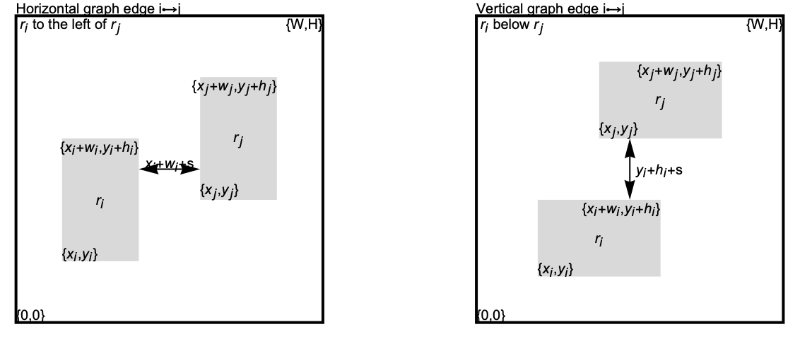
Let ![]() be the minimal spacing between rectangles. When
be the minimal spacing between rectangles. When ![]() has the edge ij, rectangle
has the edge ij, rectangle ![]() is constrained to be to the left of rectangle
is constrained to be to the left of rectangle ![]() , so
, so ![]() . When
. When ![]() has the edge ij, rectangle
has the edge ij, rectangle ![]() is constrained to be below rectangle
is constrained to be below rectangle ![]() , so
, so ![]() . Traversing the graph and accounting for rectangles that can be at the edges of the floor can be done with the following function:
. Traversing the graph and accounting for rectangles that can be at the edges of the floor can be done with the following function:
positionConstraints[g_, x_, w_, W_, s_, n_] :=
	Module[{u, l, cp, cl, cu, edgeConstraint},
	u[_] = True;
	l[_] = True;
	edgeConstraint[DirectedEdge[i_, j_]] := (
	u[i] = False;l[j] = False;x[i] + w[i] + s ≤ x[j]);
	cp = Map[edgeConstraint, EdgeList[g]];
	cl = Table[If[l[i], x[i] ≥ 0, Nothing], {i, n}];
	cu = Table[If[u[i], x[i] + w[i] ≤ W, Nothing], {i, n}];
	Join[cp, cl, cu]
	];
Given the placement graphs, the areas, ![]() and
and ![]() , the rules can be combined in a function that uses GeometricOptimization:
, the rules can be combined in a function that uses GeometricOptimization:
planFloor[{gx_, gy_}, areas_, α_, s_] :=
Block[{n = Length[areas], x, w, W, y, h, H},
If[NumberQ[area], areas = ConstantArray[area, n]];
horizontalConstraints = positionConstraints[gx, x, w, W, s, n];
verticalConstraints = positionConstraints[gy, y, h, H, s, n];
Subscript[x, all] = Array[x, n];
Subscript[w, all] = Array[w, n];
Subscript[y, all] = Array[y, n];
Subscript[h, all] = Array[h, n];
aspectConstraints = 1 / αSubscript[h, all] / Subscript[w, all]α;areaConstraints = Subscript[h, all] * Subscript[w, all] == areas;rules = GeometricOptimization[W * H, {horizontalConstraints, verticalConstraints, aspectConstraints, areaConstraints}, Flatten[{W, H, Subscript[x, all], Subscript[w, all], Subscript[y, all], Subscript[h, all]}], Tolerance -> 0.0025];
{Rectangle[{0, 0}, {W, H}] /. rules, AssociationMap[Function[Rectangle[{x[#], y[#]}, {x[#] + w[#], y[#] + h[#]}] /. rules], Range[n]]}]Here are graphs that describe relative placement for 3 rectangles such that the first is to the left of the other two and the second is below the third:
Subscript[g, x] = Graph[Range[3], {12, 13}];
Subscript[g, y] = Graph[Range[3], {23}];plan = planFloor[{Subscript[g, x], Subscript[g, y]}, {3, 1, 1}, 2, 1]Here is a function to show the plan:
showPlan[{big_, little_}] := Module[{showRectangle},
	showRectangle[key_, r : Rectangle[ll_, ur_]] := {LightGray, r, Black, Text[ToString[key], (ll + ur) / 2]};
Graphics[{{EdgeForm[Thick], FaceForm[], big}, MapThread[showRectangle, {Keys[little], Values[little]}]}]]showPlan[plan]This shows a plan for 10 rectangles with randomly assigned areas:
Subscript[g, 10x] = Graph[Range[10], {12, 13, 14, 15, 16, 17, 23, 45, 23, 25, 27, 43, 45, 47, 65, 84, 94, 104, 106, 67, 89, 810}];
Subscript[g, 10y] = Graph[Range[10], {16, 17, 18, 19, 110, 24, 29, 46, 35, 57, 96, 910}];
areas = BlockRandom[RandomReal[1, 10], RandomSeeding -> "seed"];
showPlan[planFloor[{Subscript[g, 10x], Subscript[g, 10y]}, areas, 1.5, 0.1]]Structural Optimization Problems (3)
Find a minimum-weight truss that is subjected to either a vertical load ![]() or a horizontal load
or a horizontal load ![]() . The bars of the truss are hollow pipes of inner radius
. The bars of the truss are hollow pipes of inner radius ![]() , outer radius
, outer radius ![]() and density
and density ![]() :
:
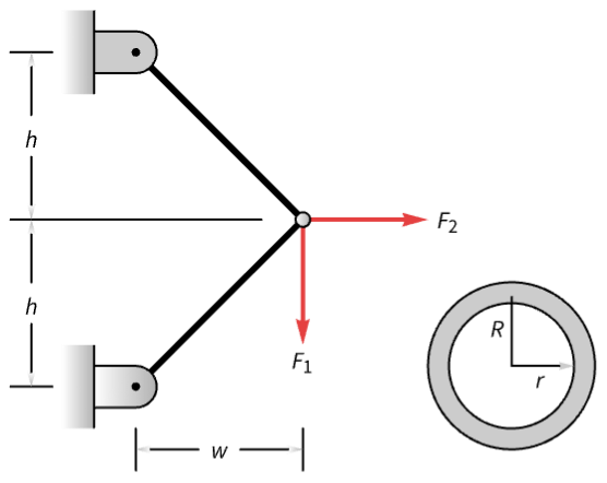
The length of the bar is defined using the height ![]() and width
and width ![]() of the truss. The cross-sectional area is
of the truss. The cross-sectional area is ![]() . The objective is to minimize weight:
. The objective is to minimize weight:
weight = 2ρ A Sqrt[h^2 + w^2];When vertical load ![]() is applied, the force in each bar is:
is applied, the force in each bar is:
verticalForceInBar = (Subscript[F, 1]Sqrt[h^2 + w^2]) / (2h);When horizontal load ![]() is applied, the force in each bar is:
is applied, the force in each bar is:
horizontalForceInBar = (Subscript[F, 2]Sqrt[h^2 + w^2]) / (2w);The total forces in the bars must not exceed maximum allowable force ![]() , where
, where ![]() is the maximum allowable stress:
is the maximum allowable stress:
forceConstraints = {2verticalForceInBar ≤ σ A, 2horizontalForceInBar ≤ σ A};The truss height ![]() and truss width
and truss width ![]() are constrained:
are constrained:
structureConstraints = {0.1 ≤ w ≤ 2, 0.1 ≤ h ≤ 2};Require that the tube has a minimum wall thickness. This can be done by requiring that ![]() with
with ![]() . The relation between bar area and radius is
. The relation between bar area and radius is ![]() but is not a monomial function. Using
but is not a monomial function. Using ![]() and the constraint
and the constraint ![]() , the resulting constraints are monomials:
, the resulting constraints are monomials:
barConstraint = {(α r)^2 - r^2 ≤ A / (2π), Sqrt[r^2 + A / (2π)] ≤ Subscript[R, max]};Specify the parameters of the truss:
params = {α -> 1.1, ρ -> 2700, σ -> 69000, Subscript[F, 1] -> 10^3, Subscript[F, 2] -> 10^3, Subscript[R, max] -> 5};Solve for ![]() to get the optimal truss:
to get the optimal truss:
res = GeometricOptimization[weight /. params, {forceConstraints,
	structureConstraints, barConstraint} /. params, {h, w, r, A}]
Recover the outer radius ![]() of the bar using
of the bar using ![]() :
:
Sqrt[(r ^ 2 + A / (2π))] /. resFind a minimum-weight truss subjected to a vertical load ![]() . The height
. The height ![]() and width
and width ![]() of the truss are known. The vertical position of joint
of the truss are known. The vertical position of joint ![]() is not known:
is not known:
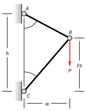
Let ![]() be the cross-sectional areas of bar
be the cross-sectional areas of bar ![]() and bar
and bar ![]() , respectively, and
, respectively, and ![]() be the density of the bar. The weight of the truss is given by:
be the density of the bar. The weight of the truss is given by:
weight = ρ(Subscript[A, 1]Sqrt[w^2 + (h - Subscript[y, b])^2] + Subscript[A, 2]Sqrt[w^2 + Subscript[y, b]^2]);Bar ![]() undergoes tension. Let
undergoes tension. Let ![]() be the tensile stress of the material. The force on bar
be the tensile stress of the material. The force on bar ![]() must not exceed the maximum allowable force:
must not exceed the maximum allowable force:
barABConstraint = (P Sqrt[w^2 + (h - Subscript[y, b])^2] / h) ≤ Subscript[σ, t]Subscript[A, 1];Bar ![]() undergoes compression. Let
undergoes compression. Let ![]() be the compressive stress of the material. The force on bar
be the compressive stress of the material. The force on bar ![]() must not exceed the maximum allowable force:
must not exceed the maximum allowable force:
barBCConstraint = (P Sqrt[w^2 + Subscript[y, b]^2] / h) ≤ Subscript[σ, c]Subscript[A, 2];params = {ρ -> 7.7, Subscript[σ, t] -> 150 10 ^ 3, Subscript[σ, c] -> 100 10 ^ 3, h -> 2, w -> 1, P -> 100};A specific instance of the geometric optimization problem can be solved for a given value of ![]() . Assuming the vertical position of joint
. Assuming the vertical position of joint ![]() must lie between a certain range, solve a range of problems:
must lie between a certain range, solve a range of problems:
res = Table[{Subscript[y, b], GeometricOptimization[weight /. params
, {barABConstraint, barBCConstraint} /. params, {Subscript[A, 1], Subscript[A, 2]}, "PrimalMinimumValue"]}, {Subscript[y, b], Subdivide[0.5, 1.5, 20]}];ListPlot[res, AxesLabel -> {"SubscriptBox[y, b]", "Weight"}]Find the specific value of ![]() that gives the minimum weight:
that gives the minimum weight:
yOpt = FindArgMin[Interpolation[res][x], {x, 0.5, 1.5}][[1]]Find the optimal cross-sectional areas and the truss weight:
GeometricOptimization[weight /. params /. Subscript[y, b] -> yOpt
	, {barABConstraint, barBCConstraint} /. params /. Subscript[y, b] -> yOpt, {Subscript[A, 1], Subscript[A, 2]}, {"PrimalMinimizerRules", "PrimalMinimumValue"}]
Design a minimum-weight cantilever beam subject to a vertical load ![]() on the free end. The beam consists of
on the free end. The beam consists of ![]() segments of unit length. Each segment has a width
segments of unit length. Each segment has a width ![]() and height
and height ![]() :
:
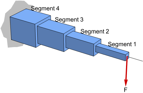
n = 16;
weight = w.h;
The load causes the beam to deflect and induces stress ![]() on each segment of the beam. The stress must be less than the maximum allowable stress
on each segment of the beam. The stress must be less than the maximum allowable stress ![]() :
:
stressConstraints = Table[6 * i * F / (Indexed[w, i] * Indexed[h, i] ^ 2) ≤ Subscript[σ, max], {i, n}];Let ![]() be the deflection at the right end of segment
be the deflection at the right end of segment ![]() . The deflection
. The deflection ![]() at the free end can be found recursively as
at the free end can be found recursively as ![]() , where
, where ![]() is the Young's modulus and the slope
is the Young's modulus and the slope ![]() . Since segment
. Since segment ![]() is fixed,
is fixed, ![]() :
:
v[n + 1] = y = 0;
Do[v[i] = (12(i - 1 / 2) * (F / (Y * Indexed[w, i] * Indexed[h, i] ^ 3))) + v[i + 1], {i, n, 1, -1}];
Do[y += 6 * (i - 1 / 3) * (F / (Y * Indexed[w, i] * Indexed[h, i] ^ 3)) + v[i + 1], {i, n, 1, -1}];
The deflection on the free end of the beam must be less than the maximum allowable deflection ![]() :
:
deflectionConstraint = y ≤ Subscript[y, max];The width, height and aspect ratios are constrained to be in a certain range:
dimensionConstraints = {0.1w20, 0.1h6, 0.1h / w5};params = {Y -> 1, F -> 0.1, Subscript[σ, max] -> 1, Subscript[y, max] -> 10};Find the dimensions of the individual segments by minimizing the weight:
res = GeometricOptimization[weight, {stressConstraints,
	deflectionConstraint, dimensionConstraints} /. params, {w∈Vectors[n], h∈Vectors[n]}]
Visualize the cantilever beam:
beamSegments = MapThread[Translate[Cuboid[{-1 / 2, -#1 / 2, -#2 / 2},
	{1 / 2, #1 / 2, #2 / 2}], {-#3, 0, 0}]&, {w, h, Range[0, n - 1]} /. res];
Graphics3D[{Opacity[0.5], beamSegments}, BoxRatios -> {3, 1, 1}]
Circuit Problems (3)
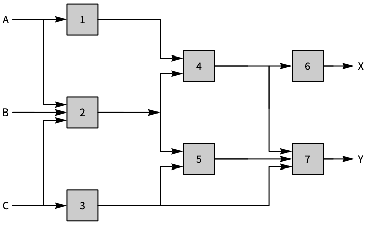
Digital circuit gate sizing: Find the optimal sizes of the gates in a given circuit subject to power and area constraint such that delay in the circuit is minimized. Consider a seven-gate circuit:
Let ![]() be a scaling factor by which each gate must be increased:
be a scaling factor by which each gate must be increased:
scalingConstraint = x1;The area taken by each gate is assumed to be proportional to the scaling factor, so the total circuit area is:
circuitArea = Total[x];The energy lost when gate ![]() transitions is proportional to the scale factor
transitions is proportional to the scale factor ![]() , the transition frequency of the gate
, the transition frequency of the gate ![]() and the energy lost
and the energy lost ![]() when the gate transitions:
when the gate transitions:
transitionFrequency = {1, 0.8, 1, 0.7, 0.7, 0.5, 0.5};
energyLost = {1, 2, 1, 1.5, 1.5, 1, 2};
powerConsumed = (transitionFrequency * energyLost).x;
Gate ![]() has input capacitance
has input capacitance ![]() except gates 6 and 7, which have input capacitance of 10:
except gates 6 and 7, which have input capacitance of 10:
inputCapacitance = Join[Table[1 + Indexed[x, i], {i, 5}], {10, 10}];Gate ![]() has a driving resistance
has a driving resistance ![]() :
:
drivingResistance = Table[1 / Indexed[x, i], {i, 7}];Gate ![]() capacitance is the sum of the input capacitances of the gates its output is connected to, except output gates 6 and 7, whose capacitance is the same as their input capacitance:
capacitance is the sum of the input capacitances of the gates its output is connected to, except output gates 6 and 7, whose capacitance is the same as their input capacitance:
connections = {{4}, {4, 5}, {5, 7}, {6, 7}, {7}, {6}, {7}};
gateCapacitance = Map[Total[inputCapacitance[[#]]]&, connections];
The delay of gate ![]() is the product of its driving resistance and the gate capacitance:
is the product of its driving resistance and the gate capacitance:
delay = drivingResistance * gateCapacitance;The objective is to minimize the worst-case delay for all combinations of paths that can be traversed in the circuit:
paths = {{1, 4, 6}, {1, 4, 7}, {2, 4, 6}, {2, 4, 7}, {2, 5, 7}, {3, 5, 6}, {3, 7}};
objective = Max@@Map[Total[delay[[#]]]&, paths]
The circuit area must be less than a specified maximum allowable area:
areaConstraint = circuitArea ≤ aMax;The power consumed must be less than a specified maximum allowable power:
powerConstraint = powerConsumed ≤ pMax;Find the minimum area for different combinations of maximum allowable area and power:
res = Table[{pMax, GeometricOptimization[objective, {scalingConstraint,
	areaConstraint, powerConstraint}, x, "PrimalMinimumValue"]}, {aMax, {25, 50, 100}}, {pMax, 10, 100, 5}];
Plot the optimal tradeoff curves:
ListLinePlot[res, ...]Find the widths of ![]() wire segments in an interconnected network in a circuit with known capacitance. There are five wire segments in the network below:
wire segments in an interconnected network in a circuit with known capacitance. There are five wire segments in the network below:
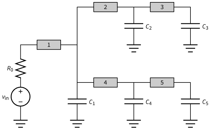
For each wire segment, the resistance ![]() and capacitances
and capacitances ![]() , where
, where ![]() , are positive constants depending on the wire properties and
, are positive constants depending on the wire properties and ![]() is the length of the wire and width
is the length of the wire and width ![]() :
:
wireResistance = Table[Subscript[R, i] -> α(l / Indexed[w, i]), {i, 5}];
wireCapacitance = Table[Subscript[S, i] -> β * l * Indexed[w, i] + γ * l, {i, 5}];
Using a ![]() model, each wire is modeled using a resistor and capacitor. The resulting network becomes a resistor-capacitor network:
model, each wire is modeled using a resistor and capacitor. The resulting network becomes a resistor-capacitor network:

The new capacitances of the model are obtained by summing the respective network capacitances with the wire capacitances ![]() :
:
rcCapacitance = {Subscript[Overscript[c, ~], 0] -> Subscript[S, 1], Subscript[Overscript[c, ~], 1] -> Subscript[c, 1] + Subscript[S, 1] + Subscript[S, 2] + Subscript[S, 4], Subscript[Overscript[c, ~], 2] -> Subscript[c, 2] + Subscript[S, 2] + Subscript[S, 4],
	Subscript[Overscript[c, ~], 3] -> Subscript[c, 3] + Subscript[S, 3], Subscript[Overscript[c, ~], 4] -> Subscript[c, 4] + Subscript[S, 4] + Subscript[S, 5], Subscript[Overscript[c, ~], 5] -> Subscript[c, 5] + Subscript[S, 5]} /. wireCapacitance;
The Elmore delay measures the delay of voltage changing and converging to a new value. The Elmore delay for each capacitor ![]() is
is ![]() , where
, where ![]() is the set of resistances between capacitors
is the set of resistances between capacitors ![]() and
and ![]() :
:
V = {...};
elmoreDelay = V.{Subscript[Overscript[c, ~], 0], Subscript[Overscript[c, ~], 1], Subscript[Overscript[c, ~], 2], Subscript[Overscript[c, ~], 3], Subscript[Overscript[c, ~], 4], Subscript[Overscript[c, ~], 5]} ;
The objective is to minimize the largest Elmore delay:
objective = Max@@elmoreDelay /. Join[wireResistance, rcCapacitance];The wire is constrained to be within a range:
wireConstraint = 1w5;The total area cannot exceed a maximum allowable area:
areaConstraint = l * Total[w] ≤ Subscript[A, max];params = {Subscript[R, 0] -> 0.1, l -> 1, α -> 1, β -> 1, γ -> 1, Subscript[A, max] -> 20, Subscript[c, 1] -> 10, Subscript[c, 2] -> 10, Subscript[c, 3] -> 10, Subscript[c, 4] -> 10, Subscript[c, 5] -> 10};GeometricOptimization[objective /. params, {wireConstraint,
areaConstraint} /. params, w∈Vectors[5]]Find the optimal doping profile of a transistor such that the base transit time is minimized. Let ![]() be the doping profile, where
be the doping profile, where ![]() is the base-width. Let
is the base-width. Let ![]() be the base transit time. A simplified model as a function of
be the base transit time. A simplified model as a function of ![]() is given by
is given by ![]() , where
, where ![]() is a constant. Let
is a constant. Let ![]() ; then the integral can be discretized using
; then the integral can be discretized using ![]() equally spaced points:
equally spaced points:
M = 40;
c = Subscript[W, B] / (M + 1);
baseTransitTime = κ c^2 Sum[Indexed[v, i]^(Subscript[γ, 2] - 1) Sum[Indexed[v, j]^1 + Subscript[γ, 1] - Subscript[γ, 2],
	{j, i, M + 1}], {i, 1, M + 1}];
The doping gradient constraint ![]() can be approximated as:
can be approximated as:
dopingGradientConstraint = Table[(1 - α c) Indexed[v, i] ≤
	Indexed[v, i + 1] ≤ (1 + α c) Indexed[v, i], {i, 1, M}];
The doping profile has upper and lower limits and specified initial and final states:
dopingProfileConstraints = {Subscript[V, min]vSubscript[V, max], Indexed[v, 1] == Subscript[V, max],
Indexed[v, M + 1] == Subscript[V, min]};params = {Subscript[V, min] -> 50, Subscript[V, max] -> 500, Subscript[γ, 1] -> 0.42, Subscript[γ, 2] -> 0.69, Subscript[W, B] -> 1, α -> 10, κ -> 1};Solve the resulting geometric optimization problem to get the optimal doping profile:
res = GeometricOptimization[baseTransitTime /. params, {dopingGradientConstraint, dopingProfileConstraints} /. params, v∈Vectors[M + 1]]ListLinePlot[v /. res, PlotRange -> All]Power Control (1)
Minimize the total power levels ![]() that
that ![]() transmitters transmit at to
transmitters transmit at to ![]() receivers:
receivers:
n = 5;
totalPower = Total[P];
The power received by receiver ![]() from transmitter
from transmitter ![]() is
is ![]() , where
, where ![]() represents the path gain from transmitter
represents the path gain from transmitter ![]() to receiver
to receiver ![]() :
:
powerReceived[G_, i_, j_] := G[[i, j]] Indexed[P, j];The signal power at receiver ![]() is
is ![]() :
:
powerAtReceiver[G_, i_] := G[[i, i]] Indexed[P, i];The interference power at receiver ![]() is the total power received from all transmitters except
is the total power received from all transmitters except ![]() ,
, ![]() :
:
interferencePower[G_, i_] := Sum[powerReceived[G, i, k],
	{k, Complement[Range[n], {i}]}];
The signal-to-interference-and-noise ratio (SINR) of the ![]()
![]() receiver/transmitter pair is given by
receiver/transmitter pair is given by ![]() , where
, where ![]() is the noise power at receiver
is the noise power at receiver ![]() :
:
S[G_ ? MatrixQ, σ_ ? VectorQ, i_Integer] := powerAtReceiver[G, i] / (σ[[i]] + interferencePower[G, i]);The SINR of any receiver/transmitter pair has a minimum threshold. To make this a posynomial constraint, take the inverse of the SINR constraints ![]() :
:
thresholdContraint[G_ ? MatrixQ, σ_ ? VectorQ] := Table[1 / S[G, σ, i] ≤ 1 / Subscript[S, min], {i, n}];The power levels have a lower and an upper limit:
powerConstraint = Subscript[P, min]PSubscript[P, max];SeedRandom[1234];
params = {G -> RandomReal[{0, 1}, {n, n}] + 2IdentityMatrix[n], σ -> ConstantArray[10, n], Subscript[S, min] -> 1, Subscript[P, min] -> 10, Subscript[P, max] -> 50};GeometricOptimization[totalPower, {thresholdContraint[G, σ],
powerConstraint} //. params, P∈Vectors[n]]Text
Wolfram Research (2020), GeometricOptimization, Wolfram Language function, https://reference.wolfram.com/language/ref/GeometricOptimization.html.
CMS
Wolfram Language. 2020. "GeometricOptimization." Wolfram Language & System Documentation Center. Wolfram Research. https://reference.wolfram.com/language/ref/GeometricOptimization.html.
APA
Wolfram Language. (2020). GeometricOptimization. Wolfram Language & System Documentation Center. Retrieved from https://reference.wolfram.com/language/ref/GeometricOptimization.html