Wolfram言語＆システムドキュメントセンター

HistogramPointDensity

HistogramPointDensity[pdata]

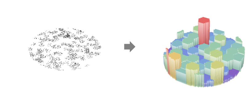
ヒストグラム点密度関数を点データ pdata について推定する．

HistogramPointDensity[pdata,bspec]

ヒストグラム点密度関数を bspec によるヒストグラムビン指定で推定する．

HistogramPointDensity[bdata,…,…]

ヒストグラム点密度関数をビン分割されたデータ bdata について推定する．

HistogramPointDensity[pproc,…,…]

ヒストグラム点密度関数を点過程 pproc について計算する．

HistogramPointDensity

HistogramPointDensity[pdata]

ヒストグラム点密度関数を点データ pdata について推定する．

HistogramPointDensity[pdata,bspec]

ヒストグラム点密度関数を bspec によるヒストグラムビン指定で推定する．

HistogramPointDensity[bdata,…,…]

ヒストグラム点密度関数をビン分割されたデータ bdata について推定する．

HistogramPointDensity[pproc,…,…]

ヒストグラム点密度関数を点過程 pproc について計算する．

詳細とオプション

点密度は点強度としても知られている．
HistogramPointDensityは，点の数が観測領域の長さ，面積，体積によってどのように変わるかを記述する関数を与える．領域上の積分は点の総数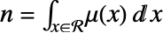である．

HistogramPointDensityは分割に基づいた点密度の推定器である．平滑化の制御にはビン指定 bspec が使われる．

ヒストグラム点密度は，一般に，非同次ポアソン(Poisson)過程または非同次性の測度を定義するために使われる．
HistogramPointDensityは，密度関数を繰り返し評価するために使えるPointDensityFunctionを返す．
点 pdata は次の形式でよい．

	{p₁,p₂,…}	点 p_i
	GeoPosition[…],GeoPositionXYZ[…],…	地理的な点
	SpatialPointData[…]	観測領域がある空間点集合
	{pts,reg}	点集合 pts と観測領域 reg

観測領域 reg は，与えられていない場合はRipleyRassonRegionを使って自動的に計算される．
ビン分割データ bdata はSpatialBinnedPointDataの形であると想定される．
点過程 pproc は次の形式でよい．
proc 厳密な式による点過程 proc

{proc,reg} シミュレーションに基づいた点過程 proc と観測領域 reg
観測領域 reg はパラメータフリーの全次元で，SpatialObservationRegionQで調べられるような有界領域である．
次の代数的・地理的ビン指定 bspec を使うことができる．

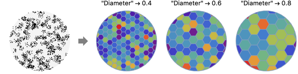
	MeshRegion[…]	セルがある明示的なMeshRegion
	"ObservationMesh"	観測領域の離散化
	{reg₁,reg₂, ...}	不連続領域の明示的なリスト
	shape	次元に依存する代数的形状
	{shape,"Count"n}	約 n 個に集約されたビン
	{shape,"Measure"ν}	近似測度 ν の集約されたビン
	{shape,"Diameter"d}	近似直径 d の集約されたビン

次は，shape の可能な設定である．
"Triangle" 2Dの三角形ビン

"Square" 2Dの正方形ビン

"Hexagon" 2Dの六角形ビン
幾何学ビンは，bspec を座標ごとに与えることで作ることもできる．

	n	n 個のビンを使う
	{w}	幅 w のビンを使う
	{min,max,w}	幅 w（min から max まで）のビンを使う
	{{b₁,b₂,…}}	ビン[b₁,b₂),[b₂,b₃),…を使う
	Automatic	ビン幅を自動的に決定する
	"name"	名前付きのビン分割メソッドを使う
	fw	fw を適用して明示的なビン指定{b₁,b₂,…}を得る
	{xspec,yspec,…}	x, y 等の異なる指定を与える

次は，使用可能な名前付きビン分割メソッドである．

	"FreedmanDiaconis"	四分位範囲の2倍をサンプルサイズの立方根で割った値
	"Knuth"	区分一様モデルの平衡尤度と事前確率
	"Scott"	平均二乗誤差を漸近的に最小化する
	"Sturges"	データ長に基づいてビン数を計算する
	"Wand"	1レベルの再帰的近似Wandビン分割

ビンはすべて観測領域と交差するように切り取られる．

例題

すべて開くすべて閉じる

例 (2)

SpatialPointDataを作成する：

Wolfram Language code: spd = SpatialPointData[RandomReal[1, {300, 2}]];

点密度を推定する：

Wolfram Language code: μ = HistogramPointDensity[spd]

点における値：

Wolfram Language code: μ[{.3, .5}]

密度推定を可視化する：

Wolfram Language code: DiscretePlot3D[μ[{x, y}], {x, 0, .95, .05}, {y, 0, .95, .05}, ExtentSize -> Full, ColorFunction -> "Rainbow"]

地理的な点のリストについてヒストグラム点密度を計算する：

Wolfram Language code:

data = GeoPosition[{{57.38695860758024, -2.082019036397938}, {64.51592745731402, 45.824927190648225}, 
  {56.6010212397469, -6.240526809704691}, {51.60678874558969, 57.27710883880354}, 
  {45.30573867042673, 15.472775964257096}, {47.62531221069711, 33.091 ... 064113254605, 6.294616072872941}, {70.14917097063635, 58.711274282407935}, 
  {53.9133525034849, 51.235121204775595}, {47.95050112387477, 50.208632516820614}, 
  {45.978247255215074, 0.000929944545532635}, {61.154927383569934, 53.20226357948661}}];

Wolfram Language code: μ = HistogramPointDensity[data, "Hexagon"]

密度を可視化する：

Wolfram Language code: μ["DensityVisualization"]

スコープ (5)

同次一変量SpatialPointDataを作成する：

Wolfram Language code:

reg = Rectangle[{0, 0}, {3, 3}];
data = SpatialPointData[RandomPoint[reg, 200], reg]

異なるビンの形を使って点密度関数を計算する：

Wolfram Language code: μ1 = HistogramPointDensity[data, "Triangle"]

Wolfram Language code: μ2 = HistogramPointDensity[data, "Hexagon"]

ランダムな場所の値を使って可視化する：

Wolfram Language code:

sample = RandomPoint[reg, 5 * 10 ^ 3];vals1 = μ1[sample];vals2 = μ2[sample];max = Max[{vals1, vals2}];
colors1 = ColorData["Rainbow"] /@ (vals1 / max);
colors2 = ColorData["Rainbow"] /@ (vals2 / max);

Wolfram Language code:

ListPlot[MapThread[Style[#1, #2]&, {sample, #}], AspectRatio -> 1, PlotStyle -> PointSize[Medium]]& /@ {colors1, colors2}

クラスタ化されたデータのヒストグラム点密度：

Wolfram Language code: data = RandomPointConfiguration[MaternPointProcess[10, 50, .1, 2], Rectangle[]];

Wolfram Language code: ListPlot[data, AspectRatio -> Automatic]

ヒストグラム点密度をデータから計算する：

Wolfram Language code: μ = HistogramPointDensity[data]

可視化：

Wolfram Language code:

Show[ContourPlot[μ[{x, y}], {x, 0, 1}, {y, 0, 1}, ContourStyle -> None, ColorFunction -> "SolarColors"], ListPlot[data, PlotStyle -> Black]]

ハードコア過程についてのヒストグラム点密度：

Wolfram Language code:

reg = Disk[{0, 0}, 3];
data = RandomPointConfiguration[HardcorePointProcess[10, r = 0.2, 2], reg, Method -> {Automatic, "LengthOfRun" -> 10 ^ 4}];

Wolfram Language code: ListPlot[data, AspectRatio -> Automatic]

さまざまなビンの直径についてのデータからヒストグラム点密度を計算する：

Wolfram Language code:

diams = {r, 2r, 3r};
μ = HistogramPointDensity[data, {"Square", "Diameter" -> #}]& /@ diams;

可視化：

Wolfram Language code:

Table[Show[ContourPlot[μ[[k]][{x, y}], {x, -3, 3}, {y, -3, 3}, ContourStyle -> None, ColorFunction -> "PearlColors", PlotLabel -> Row[{"bandwidth = ", diams[[k]]}]], ListPlot[data, PlotStyle -> Black]], {k, 3}]

ビンの形状指定を比較する：

Wolfram Language code: sp = SpatialPointData[RandomReal[1, {50, 2}], Rectangle[]];

メッシュ領域と多角形合成領域を定義する：

Wolfram Language code: mesh = [image];

Wolfram Language code: polygonlist = MeshPrimitives[mesh, 2];

密度を計算する：

Wolfram Language code:

pfs = Table[HistogramPointDensity[sp, type], {type, {"MeshRegion", "AggregatedMeshRegion", "Hexagon", "Square", "Triangle", mesh, polygonlist}}];

Wolfram Language code: types = {"MeshRegion", "AggregatedMeshRegion", "Hexagon", "Square", "Triangle", "mesh", "polygonlist"};

密度を可視化する：

Wolfram Language code: MapThread[Show[Labeled[#1["DensityVisualization"], #2], ImageSize -> 110]&, {pfs, types}]

地球表面に許可されたビン指定：

Wolfram Language code: pts = SpatialPointData@RandomGeoPosition[Entity["Country", "Italy"], 100];

Wolfram Language code: GeoListPlot[pts["Points"]]

密度を計算する：

Wolfram Language code:

pfs = Table[HistogramPointDensity[pts, type], {type, {"MeshRegion", "AggregatedMeshRegion", "Hexagon", "Square", "Triangle"}}];

可視化する：

Wolfram Language code: GraphicsRow@Table[Show[pf["DensityVisualization"], ImageSize -> 100], {pf, pfs}]//Quiet

アプリケーション (1)

ニューヨーク市におけるネズミの目撃データを取得する：

Wolfram Language code: tab = Tabular[ResourceData["NYC Rat Sightings"]]

列キーをリストして場所の列を求める：

Wolfram Language code: ColumnKeys[tab]

地理位置を抽出し，欠落しているものは削除してSpatialPointDataを作成する：

Wolfram Language code: pts = DeleteMissing[Normal[tab[All, "GeoLocation"]]];locs = SpatialPointData[pts]

ヒストグラム点密度を計算する：

Wolfram Language code: density = HistogramPointDensity[locs]

ニューヨーク市におけるネズミの目撃情報が多い地域を，以下の場所のサンプルで可視化する：

Wolfram Language code:

pos = RandomSample[pts, 3000];
vals = density[pos];

Wolfram Language code:

PointValuePlot[pos -> vals, ColorFunction -> "Rainbow", PlotStyle -> PointSize[Small], GeoBackground -> "VectorMonochrome"]

特性と関係 (1)

HistogramPointDensityはビンの高さ指定が"Intensity"であるHistogramと関連している：

Wolfram Language code: data1 = RandomPointConfiguration[PoissonPointProcess[100, 1], Interval[{-1, 1}]];

ヒストグラム点密度の計算でビンの幅を指定する：

Wolfram Language code: μ1 = HistogramPointDensity[data1, {.1}]

密度関数と同じビン幅の強度Histogramを比較する：

Wolfram Language code: Show[Histogram[data1, {.1}, "Intensity"], Plot[μ1[{x}], {x, -1, 1}]]

2Dデータについて：

Wolfram Language code: data2 = RandomPointConfiguration[PoissonPointProcess[100, 2], Rectangle[]];

Wolfram Language code: ListPlot[data2]

ヒストグラム点密度を計算する：

Wolfram Language code: μ2 = HistogramPointDensity[data2, {.1}]

密度関数のプロットとデータのHistogram3Dを比較する：

Wolfram Language code:

μplot = DiscretePlot3D[μ2[{x, y}], {x, 0, 1, .1}, {y, 0, 1, .1}, ExtentSize -> Right, ColorFunction -> "Rainbow", PlotRange -> {{0, 1}, {0, 1}, All}];

Wolfram Language code: h = Histogram3D[data2, {.1}, "Intensity", ColorFunction -> (ColorData["Rainbow"][Rescale[#, {0, 1}, {0.25, 1}]]&)];

Wolfram Language code: {μplot, h}

Top

その他のラーニングリソース

テクニカルサポート

データサイエンス，金融，ビジネス

工学

科学とテクノロジー

教育のためのテクノロジー

教育イニシアチブ

使い始める

Grow Your Skills

Wolframと繋がる

大人用の教育プログラム

若者のための教育プログラム

読む

HistogramPointDensity

詳細とオプション

例題

例 (2)

スコープ (5)

アプリケーション (1)

特性と関係 (1)

テキスト

CMS

APA

BibTeX

BibLaTeX

	proc	厳密な式による点過程 proc
	{proc,reg}	シミュレーションに基づいた点過程 proc と観測領域 reg

	"Triangle"	2Dの三角形ビン
	"Square"	2Dの正方形ビン
	"Hexagon"	2Dの六角形ビン

HistogramPointDensity

詳細とオプション

例題

例 (2)

スコープ (5)

アプリケーション (1)

特性と関係 (1)

関連項目

関連するガイド

履歴

テキスト

CMS

APA

BibTeX

BibLaTeX